We ran over 4000 scaling experiments on up to 512 GPUs and measured throughput (size of markers) and GPU utilization (color of markers). Note that both are normalized per model size in this visualization.
Thousands of GPUs humming in perfect harmony. That's what it takes to train today's most powerful AI models – a symphony of computing power that until recently was the exclusive domain of elite research labs. Open source has transformed this landscape, but not completely. Yes, you can download the latest Llama or DeepSeek models. Yes, you can read their technical and experiment reports. But the most challenging part – the training code, the knowledge and techniques necessary to coordinate GPUs to train these massive systems – remains shrouded in complexity and spread around a series of disconnected papers and often private codebases.
This open-source book is here to change that. Starting from the basics, we'll walk you through the knowledge necessary to scale the training of large language models from one GPU to tens, hundreds and even thousands of GPUs, illustrating theory with practical code examples and reproducible benchmarks.
As the size of the clusters used to train these models grew, various techniques such as data parallelism, tensor parallelism, pipeline parallelism or context parallelism as well as ZeRO or kernel fusion have been invented to makes sure that GPUs are highly utilized at all times. This significantly reduces training time and makes the best use of this expensive hardware. Even more, as the challenge of scaling up AI training goes beyond just building the initial models and teams have found that fine-tuning large models on specialized data often produces the best results, generally involving the same distributed training techniques. In this book we'll progressively go over all of these techniques –from the simplest to the most refined ones– while keeping a single story-line to understand where each method comes from.
We'll assume you have some simple basic knowledge about current LLM architecture and are roughtly familiar with how deep learning model are trained, but you can be generally new to distributed training. If needed, the basics of model training can be found in great courses found at DeepLearning.ai or on the PyTorch tutorial sections. This book can be seen as the second part of a trilogy following our first blog on processing data for pre-training, the so-called “FineWeb blog post”. Having read both blog posts, you should have almost all the core knowledge needed to fully understand how how performing LLMs are being built nowadays, just missing some final spices regarding data mixing and architecture choices to complete the recipe (stay tuned for part three…).
The book is built on the following three general foundations:
Quick intros on theory and concepts: before diving into code and experiments, we want to understand how each method works at a high level and what its advantages and limits are. You’ll learn about which parts of a language model eat away your memory and when during training it happens. You’ll learn how we can solve memory constraints by parallelizing the models and increase the throughput by scaling up GPUs. As a result you'll understand how the following widget to compute the memory breakdown of a transformer model works:
Memory usage breakdown
(Don't worry if you have no idea what's happening in this widget. That's why we're here.)
While this widget gives a theoretical breakdown we also made the following tool that can be used to predict the memory usage during a training run:

Clear code implementations: theory is one thing, but we discover all kinds of edge cases and important details when we implement something. That’s why we link to implementation references where possible. Depending on the case, we’ll use two code references:
-
the picotron repository is built for education, thus it implements concepts usually in single, self-contained short files.
-
On the other hand, to look at production ready code, we’ll refer to the nanotron implementations which is a production training codebase used at Hugging Face.
Real training efficiency benchmarks: Finally, how to actually scale your LLM training depends on your infrastructure, such as the kind of chips, interconnect etc., and we can’t give a single unified recipe. What we will give though is a way to benchmark several setups and it is what we have done on our cluster! We ran over 4100 distributed experiments (over 16k including test runs) with up to 512 GPUs to scan many possible distributed training layouts and model sizes.
As you can see, there’s a lot of ground to be covered. Before getting into the trenches of distributed training let’s take a quick high level look on the challenges we'll cover in the book.
High level overview
All the techniques we'll cover in this book tackle one or several of the following three key challenges, which we'll keep bumping into throughout the book:
- Memory Usage: it's a hard limitation - if a training step doesn't fit in memory, training cannot proceed
- Compute Efficiency: we want our hardware to spend most time computing, so we need to reduce time spent on data transfers or waiting for other GPUs to perform work.
- Communication overhead: we want to minimize communication overhead as it keeps GPUs idle. To achieve this we will try to make best use of intra-node (fast) and inter-node (slower) bandwidths as well as overlap communication with compute as much as possible.
In many places we'll see that we can trade one of these (computation, communication, memory) for another (e.g. recomputation or Tensor Parallelism). Finding the right balance is key to scaling training.
As this book is very extensive, we've made a cheatsheet to help you navigate the book and get the general take-away. Keep it close to your heart as you navigate these stormy waters!

First Steps: Training on one GPU
If you fancy adding a podcast feeling to your reading experience, feel free to listen to the NotebookLM hosts discussing the first sections of this book as you're reading along.
Let’s start by quickly reviewing the very basics of model training before we start to scale to many GPUs. When a model is trained on a single GPU, the training typically consists of three steps:
- a forward pass which passes inputs through the model to yield its outputs,
- a backward pass to compute the gradients, and
- an optimization step using the gradients to update the parameters
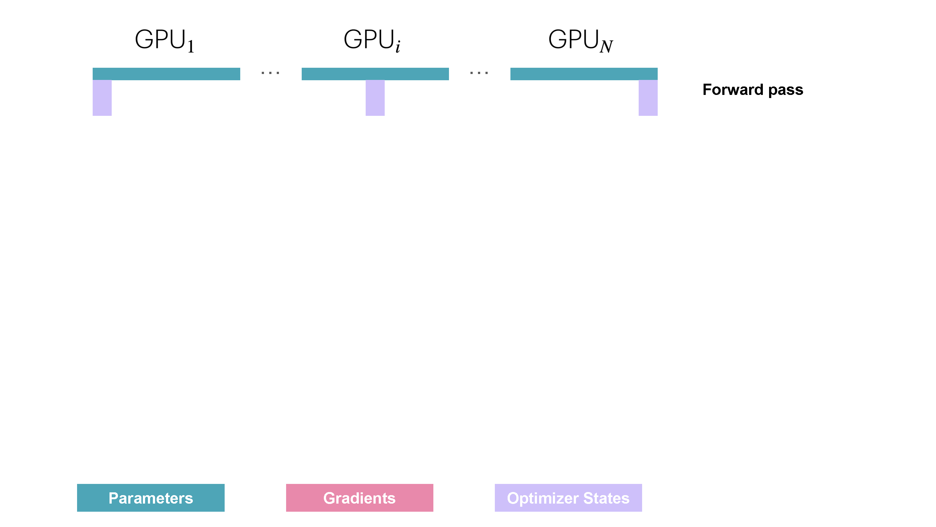
It looks generally like this:
Hover over the network elements to see their details
In this figure, the boxes on the top line can be seen as successive layers inside a model (same for the last line). The red boxes are the associated gradients for each of these layers, computed during the backward pass.
The batch size (
A small batch size can be useful early in training to quickly move along the training landscape reaching an optimal learning point. However, further along the model training, small batch sizes will keep gradients noisy and the model may not be able to converge to the most optimal final performances. At the other extreme, a large batch size while giving very accurate gradient estimations will tend to make less use of each training token rendering convergence slower and potentially wasting compute. You can find a nice early discussion of this topic in OpenAI’s paper on large batch training
Batch size also affects the time it takes to train on a given text dataset: a small batch size will require more optimizer steps to train on the same amount of samples. Optimizer steps are costly (in compute time) and the total time to train will thus increase compared to using a larger batch size. This being said, note that the batch size can often be adjusted quite largely around the optimal batch size without major impact on the performance of the model, i.e. the sensitivity of final model performances to the exact batch size value is usually rather low around the optimal batch size.
In the LLM pretraining community, batch sizes are commonly reported in terms of tokens rather than in number of samples (
In the simplest case, training on a single machine, the
From here onward we’ll show the formulas for the batch size in terms of samples but you can always get its token-unit counterpart by multiplying it with the sequence length.
A sweet spot for recent LLM training is typically on the order of 4-60 million tokens per batch. The batch size as well as the training corpus have been steadily increasing over the years: Llama 1 was trained with a batch size of ~4M tokens for 1.4 trillion tokens while DeepSeek was trained with a batch size of ~60M tokens for 14 trillion tokens.
And our first challenge is already coming ahead when scaling the training of our model to these large batch sizes: out-of-memory issues. What should we do when our GPU doesn’t have enough memory to hold a full batch of our target batch size?
Let’s start by quickly understanding what led to our out-of-memory issue in the first place. This will help us gain some useful intuitions on the memory requirements for training a model.
Memory usage in Transformers
When training a neural network model, one stores several items in memory:
- Model weights
- Model gradients
- Optimizer states
- Activations needed to compute the gradients
📝 Note
You would think for a model you could compute the memory requirements exactly but there are a few additional memory occupants that make it hard to be exact:
- CUDA Kernels typically require 1-2 GB of GPU memory, which you can quickly verify by running
import torch; torch.ones((1, 1)).to("cuda")and then checking the GPU memory withnvidia-smi. - Some rest memory usage from buffers, intermediate results and some memory that can’t be used due to fragmentation
These items are stored as tensors which come in different shapes and precisions. The shapes are determined by hyper-parameters such as batch size, sequence length, model hidden dimensions, attention heads, vocabulary size, and potential model sharding as we’ll see later. Precision refers to formats like FP32, BF16, or FP8, which respectively require 4, 2, or 1 byte to store each single value in the tensor. We will have a full discussion of the different precisions and their trade-offs in the Mixed Precision Training section, for now let's just keep in mind that the memory requirements for these various format will be different and that will impact the memory usage of the items we need to store.
So how can I quickly determine memory usage from these variables? One simple way is to do this empirically and just measure it.
Profiling the memory usage
Using the Pytorch profiler we can understand how memory is allocated throughout training. We can see that memory utilization is not a static thing but varies a lot during training and during a training step:
Clearly the first step looks very different from the subsequent ones, but let’s first have a look at the general anatomy of a step: first the activations increase quickly as we do the forward pass, then during the backward pass the gradients build up and as the backward pass propagates, the stored activations used to compute the gradients are progressively cleared. Finally, we perform the optimization step during which we need all the gradients and then update the optimizer states before we start the next forward pass.
Why does the first step looks different: the activations increase quickly and then plateau for a while. In this first step the torch cache allocator does a lot of preparation preparing memory allocations to speed up the subsequent steps so that they don’t require searching for free memory blocks afterwards (see Zach’s blog). After the first step we also see the optimizer states appearing which generally offset the memory usage for further training steps.
Now that we’ve a first view of memory, let’s see how scaling up training is often a question of maximizing compute efficiency while keeping the memory requirements of these various items (activations, parameters, gradients, optimizer states) within the memory constraints of the GPUs.
Weights/grads/optimizer states memory
Let's start with the first 3 items in our list: the model’s weights, gradients and optimizer states. We can actually pretty easily estimate the memory needed for them.
For a simple transformer LLM the number of parameters is given by the following formula:
In that equation,
Memory requirements for the parameters and gradients are simply the number of parameters multiplied by the number of bytes per parameter. In good old-fashioned full precision (FP32) training both parameters and gradients require 4 bytes while the optimizer, if we use Adam, requires the momentum and variance to be stored, which adds another two 4 bytes per parameter. In summary:
Now let’s have look how things change if we use a lower precision. For stability reasons (see the mixed-precision training section below) we often don't use full low precision training but a mix of higher and lower precision called "mixed precision"
Here’s the summary:
📝 Note
Some libraries store grads in fp32 which would require an additional bf16 is lossy for smaller values and we always prioritize stability. See this DeepSpeed issue for more information.
📝 Note
The FP32 copy of parameters (
Interestingly, mixed precision itself doesn’t save overall memory as it just distributes the memory differently across the three components, and in fact adds another 4 bytes over full precision training if we accumulate gradients in FP32. It’s still advantageous as computing the forward/backward passes in half precision allows us to (1) use optimized lower precision operations on the GPU which are faster and (2) reduces the activation memory requirements during the forward pass which is a large part of the memory usage as we saw on the graph above and below.
Let’s get a sense of how much general memory we need for a model (full and mixed precision giving the same overall value):
| Model parameters | FP32 or BF16 w/o FP32 grad acc | BF16 w/ FP32 grad acc |
|---|---|---|
| 1B | 16 GB | 20 GB |
| 7B | 112 GB | 140 GB |
| 70B | 1120 GB | 1400 GB |
| 405B | 6480 GB | 8100 GB |
As we can see, as soon as we reach 7B (!), weights and optimizer requirements already starts to add up significantly and exceed the size of a typical GPU memory, e.g. 80GB for a H100 GPU.
But for now, let’s start with models which still fit in a single GPU, take a look at the last big contributor to our memory budget: the activation memory.
Activations memory
Activation memory is a bit more complex to compute than the weights, gradients and optimizer states, in part because it depends on the inputs of the model. If you’re unsure why we even need to store activations for the backward pass, this reference is a good quick refresh. After a careful inspection of how backward pass is computed we can estimate the total memory required for the activations in mixed precision and we arrive at the following equation:
Here
For the exact derivation of the numbers, you can follow this original NVIDIA paper on recomputation
An interesting observation here is that memory usage is not static for a given model; rather, it scales linearly with the batch size and quadratically with the sequence length. This means the activation memory is the part which will blow up when we increase our batch size or train with longer sequences. We can use this equation to look at how memory usage changes for various sequence lengths for example for Llama models (bs=1):
This graph tells a striking story: for short sequences (or similar for small batch-sizes), activations are almost negligible, but starting at around 2-4k tokens they come to take a significant amount of memory while parameter, gradient and optimizer states usage (that we’ll discuss later) stays roughly independent of the sequence length and batch size.
For large input tokens (a.k.a large batch-sizes/sequences), activations become by far the largest memory burden.
Is there a way to tame this “activation explosion”? Good question, reader!
It’s time to explain our first technique – called activation recomputation– which will help us cap activation memory footprint. An essential tool in today’s large model training toolbox.
Activation recomputation
The general idea behind activation recomputation – also called gradient checkpointing or rematerialization – is to discard some activations during the forward pass to save memory and spend some extra compute to recompute these on the fly during the backward pass. Without recomputation, we store every hidden state between two learnable operations (e.g. feed-forward, layernorm etc.), such that we can use them during the backward pass to compute gradients. When we use recomputation we typically will only store activations at a few key points along the model architecture, discard the rest of activations and recompute them on the fly during the backward pass from the nearest saved activations, basically performing again a sub-part of the forward pass to trade off memory for compute. It generally looks like this:
Hover over the network elements to see their details
There are several strategies to select key activations to store:
- Full: We checkpoint activations at the transition point between each layer of the Transformer model. This is usually called the
fullstrategy since it requires a forward pass through each layer essentially adding a full forward pass during the backward pass. This strategy saves the most memory but is the most expensive one in terms of compute. It generally increases the compute cost and time by up to 30-40% which is very noticeable. - Selective: In general we can do better than full. The authors of the recomputation paper
did a detailed analysis studying which activations grow the largest and have the cheapest recomputation cost in terms of FLOPs. Turns out that the attention computations fall in that category, and thus we can usually discard them and focus on checkpointing the expensive feedforward computations. For a GPT-3 (175B) model this means 70% activation memory reduction at a 2.7% compute cost.
Let’s see how drastically recomputation strategies can in practice reduce the memory footprint and how selective recomputation strikes a nice balance between memory saving and recomputation cost:
Another trend that's clearly visibile here is how the activations for long sequences play a bigger role for smaller models, so the effect of recomputation becomes even more noticeable.
📝 Note
When you’re measuring how efficient your training setup is at using your GPU/TPU/accelerator, you usually want to take recomputation into account to compute total FLOPS (Floating point operations per second) and compare it to theoretical maximum FLOPS of the GPU/TPU/accelerator. Taking recomputation into account when calculating FLOPS for a training step gives a value called “hardware FLOPS” which is the real number of operations performed on the accelerator. Dividing this number by the duration of the training step and the maximum accelerator FLOPS yields the Hardware FLOPS Utilization (HFU).
However, what really matters at the end of the day is the start-to-end time needed to train a model on a given dataset. So when comparing various GPU/TPU/accelerator together, if one of these accelerator provide for instance enough memory to skip recomputation and thus perform less operation per second (lower HFU) but for a faster training, it should be rewarded not punished. Thus, an alternative is to compute what is called Model FLOPS Utilization (MFU) which, in contrast to HFU, only takes into account the required operations for the forward+backward passes through the model, and do not include recomputation in the measured FLOPs. This value is thus more specific to the model than the training implementation.
Most training frameworks these days use FlashAttention (that we cover further below) which integrate natively activation recomputation in its optimization strategy by recomputing attention scores and matrices in the backward pass instead of storing them. Thus most people using Flash Attention are already making use of selective recomputation.
As you’ve now understood, activation recomputation increases the number of FLOPs slightly due to recomputation, while it significantly reduces memory access overhead.
This trade-off is particularly advantageous on hardware with small high-speed memory, like GPUs, as accessing memory is typically slower than performing computations. Despite the additional operations involves, the overall effect is thus often faster computation as well, in addition to the much lower memory footprint.
Now that we’ve learned about recomputation, we can tame the activations memory usage as we saw in the above graphs!
However, activations still bears a linear dependance on the batch size and all our profiles in the barplots above were using bs=1 so as we move to larger batch sizes it might become an issue again. Do not despair as we have a second tool in our box - gradient accumulation to the rescue!
Gradient accumulation
Gradient accumulation is a very straightforward method to avoid memory explosion which consists in splitting our batch into micro-batches. We'll perform forward and backward passes successively on each micro-batch, compute the gradients, and, as the name suggests, sum the gradients of all micro-batch before we perform an optimizer step. In practice, the optimization step is conducted not on the sum but on the average of the gradients, so that the result is independent of the number of gradient accumulation steps.
Let’s call the batch size for each forward pass the micro batch size (mbs). We’ll refer to the overall batch size between each optimizer step as the global batch size (gbs). If we do one optimizer step for each 8 forward/backward passes, the global batch size will be 8 times the micro batch size.
What we now call global batch size thus corresponds to what we’ve called up to now just batch size for simplicity (we now make our terms more precise to avoid ambiguity).
With gradient accumulation the global batch size can be simply computed as follows:
Gradient accumulation allows us to effectively increase our batch size up to infinity (and beyond!) while the memory footprint stays constant. Gradient accumulation is also compatible with activation recomputation for further memory reduction.

Gradient accumulation allows us to reduce memory of activations which grow linearly with batch size by computing only only partial, micro-batches.
One drawback however, is that gradient accumulation requires multiple consecutive forward/backward passes per optimization step thereby increasing the compute overhead and slowing down training. No free lunch!
But if you’ve carefully followed, you probably noticed that the forward/backward passes for each micro-batch can actually be run in parallel. Forward/backward passes are independent from each other, with independent input samples being the only difference. Seems like it’s time to start extending our training to more than one GPU!
Before that, let's quickly see how we can vizualise computation and communication with a short tour of one of the most useful tool in the distributed training toolbox: the profiler. This tool will be extremely useful to understand and validate how communications between GPUs and compute are happening and where bottlenecks are.
Profiling GPU compute and communication
PyTorch's profiler allows us to trace and visualize exactly what's happening on both CPU and GPU during training. It's natively integrated in PyTorch. Let's see how to use it:
This generates a trace that we can visualize in TensorBoard or Chrome's trace viewer. The trace shows:
- CPU thread launching kernels asynchronously to GPU
- Multiple CUDA streams handling compute and communication in parallel
- Kernel execution times and memory allocation

Example trace showing CPU thread launching kernels asynchronously to GPU, with compute kernels and communication happening in parallel across different CUDA streams
The trace helps identify bottlenecks like:
- Sequential compute and communication that could be overlapped
- Idle GPU time waiting for data transfers
- Memory movement between CPU and GPU
- Kernel launch overhead from CPU
Understanding these patterns is crucial for optimizing distributed training performance. For example, the trace would clearly show if gradient synchronization is properly overlapped with backward computation as we'll discuss later.
Now let’s get a larger workstation 🖥️ with a couple of GPUs and start investigating our first scaling technique called data parallelism which –as we'll see– is just a parallel version of gradient accumulation.
Data Parallelism
To add a podcast feeling to your reading experience, feel free to listen to the NotebookLM hosts discussing the following sections of this book as you're reading along.
The idea behind data parallelism (DP) is to replicate the model on several GPUs (we call the replica's “model instances”) and run forward and backward passes on different micro batches of data in parallel for each GPU, hence the name Data Parallelism. You've probably already seen Data Parallelism in simple training examples but as you'll soon see we'll dive quite deeper in this section so stay tuned even if you know the general approach.

Using a different micro batch for each GPU means we’ll have different gradients in each GPU, so to keep the model instances in sync across different GPUs, the gradients from the model instances will be averaged using an operation called “all-reduce”, which happens during the backward pass, before the optimizer step.
This involves our first “distributed communication” primitive: all-reduce which handles the synchronization and communication between GPU instances and nodes.

A naive DP implementation would just wait for the backward pass the finish so that we have all gradients, then it triggers an all-reduce over all DP ranks, to sync these gradients. But such an sequential steps of computation followed by communication is A BIG NO! Because we don’t want our GPUs to stay idle while communication is happening, like on the above graph.
Instead we should try to overlap communication and computation whenever possible so that they happen at the same time as much as possible.
Let’s see three optimizations that allow us to do much better than our naive first implementation!
First optimization: Overlap gradient synchronization with backward pass
The main drawback of the naive DDP approach we’ve just described is that after the backward pass (computation), we have to wait for gradient synchronization (communication) before updating the parameters. Could we overlap this communication with our computation? The answer is yes!
As shown in the figure above, the gradients (red boxes) for a layer can be gathered and summed even before the gradients from earlier layers (red boxes to the left) have been computed. For example, as soon as the backward pass of the last layer is complete (last box on the right), those gradients can already be gathered and summed while the backward computations continue for earlier layers, moving toward the left.

This can be achieved in pytorch by attaching an all-reduce hook function to each parameter. An all-reduce operation is triggered as soon as the gradient for that parameter is ready, while gradients for other parameters are still being computed. This approach overlaps most of the all-reduce operations with gradient calculations, thereby improving efficiency. Here's a simple function to attach a hook:
Overlapping computation and communication reduces the time spent waiting for gradient synchronization across the entire model. Gradient synchronization can occur (at least partially) in parallel with backward pass, significantly speeding up data parallelism. Here's a full implementation of naive DP with synchronization overlap:
👉 Naive DP implementation with overlap in Picotron (Click to expand)
This is our first example of “overlapping computation and communication” which we will discuss several times in this blog post and is an essential technique to maximal scaling efficiency. But we can improve the efficiency even further!
Second optimization: Bucketing gradients
GPU operations are usually more efficient when performed on large tensors rather than having many operations running on smaller tensors. This is also true for communication operations. Thus, we can advantageously group gradients into buckets and launch a single all-reduce for all the gradients within the same bucket instead of performing independent all-reduce for each gradient. It will generally look like the following:

Think of it like packing items into boxes before shipping. It's more efficient to send a few big boxes than many small ones. By performing a single all-reduce operation for each bucket, we can significantly reduce communication overhead and speed up the communication operation.
Here's a code implementation with bucketing:
👉 Bucket DP implementation in Picotron (Click to expand)
Third optimization: Interplay with gradient accumulation
Finally, as we’ve seen before, gradient accumulation works by performing multiple forward and backward passes before updating the parameters with optimizer.step(). When combining gradient accumulation with data parallelism, we should be careful when we want to synchronize gradients.
In a naive version, an all-reduce operation is automatically triggered after each backward pass during the accumulation, which is sub-optimal as a single reduce after the final step would have the same effect while reducing overhead.
In PyTorch, this is typically solved by adding a model.no_sync() decorator, which disables gradient synchronization, on the backward passes which don’t need reduction.
📝 Note
When performing communication operations, tensors must be contiguous in memory to avoid redundant memory copies. To perform this optimally, we often pre-allocate continuous buffers of the size of activations or model parameters specifically for communication. While this speed up communication, it also contributes in part to the peak memory usage during training.
Now let's have a look what that means for the global batch size.
Revisit global batch size
We can update our batch size equation with our newly added Data Parallelism and Gradient Accumulation parameters:
Here
Given a targeted global batch size, we can thus trade gradient accumulation steps for data-parallel processes to speed up training.
In practice, people tend to maximize the number of data-parallel nodes (DP) over gradient accumulation as much as possible since it's inherently parallel, unlike the sequential nature of gradient accumulation. Gradient accumulation is then added on top of data parallelism to achieve the target global batch size when scaling data parallelism alone is not sufficient before you run out of GPUs.
Being able to distribute the training over different samples gives us a first dimension of parallelization, thus making this 1D parallelism (we’ll progressively cover 4 more dimensions).
Our journey up to now
Let’s quickly summarize how to setup our first 1D parallel training with a draft recipe for an optimal data-parallel setup:
- We should first determine the best (global) batch size in tokens (
GBST) either by consulting literature or running experiments measuring model convergence. - We then select a sequence length for training, again by either consulting literature or running experiments. Generally, 2-8k tokens work reliably well for the evaluations we have today (we won’t dive in training recipes here but teams usually increase the sequence at the end of the training, adding some longer-context data samples in the mix to reach the longer context size of today).
- We now know the batch size (gbs). We can find the maximum local batch size (mbs) on a single GPU by increasing the local batch size until we run out of memory.
- Finally, we determine the number of available GPUs for our target DP. The ratio of GBS to DP gives us the remaining number of gradient accumulation steps needed for the desired GBS.
If the gradient accumulation ratio is lower than one, i.e. we have too many GPUs a.k.a GPU-rich 🤑 (!), we can either choose to not use all our GPUs, explore a larger global batch size or test if a lower MBS will speed up training. In the latter case we’ll end up prioritizing throughput over individual GPU compute efficiency, using a smaller MBS than possible in order to speed up training.
Time to take a concrete example: Let’s say we want to train a recent model with a GBS of 4M tokens and a sequence length of 4k. Our batch size will thus be 1024 samples (we pick the closest powers of two). Let's assume we observe that a single GPU can only fit MBS=2 in memory and we have 128 GPUs available for training. This means with 4 gradient accumulation steps we’ll achieve our goal of 1024 samples or 4M tokens per training step. Now what if we suddenly have 512 GPUs available? We can achieve the same GBS and thus identical training by keeping MBS=2 and setting gradient accumulation steps to 1 and achieve faster training!
📝 Note
Bear in mind that at the 512+ GPUs scale, depending on the network used, the communication operations will start to be bound by ring latency (time required for a signal to propagate once around the ring) which means we can no longer fully overlap the DP communications. This will decrease our compute efficiency and hit our throughput. In this case we should start exploring other dimensions to parallelize on.
While data parallelism nicely overlaps the all-reduce gradient synchronization with backward computation to save time, this benefit starts to break down at large scales. Why? Because as we add more and more GPUs (hundreds or thousands), the overhead of coordinating between them grows significantly and the network requirements are becoming too large for the benefits. As a result, our setup will become less and less efficient which each additional GPU we add to the system.
Let's see this happening in practice with some benchmark:
We see that above some limit, our throughput starts to drop quite significantly while the memory usage per GPU stays constant and is not affected by adding more DP ranks.
Data parallelism was our first (simple) strategy to scale training across more GPUs. This technique works like gradient accumulation but parallelizes the forward and backward passes on micro batches, thus increasing throughput!
The keen reader has already probably noted however that this assumes that we can fit at least one input sample forward pass (mbs=1) into our GPU memory. This is not always the case! As we can see, larger models don’t fit into a single GPU, even with activation recomputation activated:
We've also seen that Data Parallelism starts to have some limiting communication overhead above a certain level of scaling. Do we have other options for these larger models or large batch-size? We do have some solutions thankfully. They will involve either move some tensors to the CPU or split the weights/gradients/optimizer-states tensors across GPUs devices! Let's start diving in them.
There are two main approaches to splitting: parallelism (tensor, context, or pipeline parallelism) and sharing (DeepSpeed Zero or PyTorch FSDP). Both approaches are somewhat orthogonal and can actually be combined!
The sharing paradigm is closely related to DP so we’ll have a look at it first by investigating the ZeRO method!
ZeRO (Zero Redundancy Optimizer)
In this section we will introduce DeepSpeed ZeRO (Zero Redundancy Optimizer), a memory optimization technology designed to reduce memory redundancies in LLM training.
While Data Parallelism is an efficient way to scale training, the naive replication of optimizer states, gradients, and parameters across each DP rank introduces a significant memory redundancy. ZeRO eliminates memory redundancy by partitioning the optimizer states, gradients, and parameters across the data parallel dimension, while still allowing computation with the full set of parameters. This sometimes requires more communications between DP ranks which may or may not be fully overlapped as we’ll see next!
This approach is organized into three possible optimization stage of ZeRO:
- ZeRO-1: optimizer state partitioning
- ZeRO-2: optimizer state + gradient partitioning
- ZeRO-3 (also called FSDP for “Fully-Sharded Data Parallelism”): optimizer state + gradient + parameter partitioning
You might be missing the activations among the things we can shard. Since each DP replica of the model receives a different micro-batch the activations on each DP rank also differ so they are not duplicated and thus can’t be sharded!
Let’s have a closer look how much we can save with the partitioning of each ZeRO stage!
Memory usage revisited
You likely remember from our previous section the memory usage of optimizer states, gradients, and parameters during a standard training. Let's call our model's parameters count
- Model’s parameters (half precision i.e. bf16/fp16):
2\Psi - Model’s gradients (half precision i.e. bf16/fp16):
2\Psi - Model’s parameters in fp32 and optimizer states:
4\Psi + (4\Psi + 4\Psi) - Model’s gradients in fp32:
4\Psi (optional, only accounted if we want to accumulate grads in fp32)
If we don’t accumulate gradients in fp32 this gives us a total memory consumption of
The idea of ZeRO is to shard these objects across the DP ranks, each node only storing a slice of the items which are reconstructed when and if needed, thereby dividing memory usage by the data parallel degree

Here
Let’s explain this graph and it’s values by exploring how each ZeRO stage works. We’ll start with ZeRO-1.
ZeRO-1: Partitioning Optimizer States
In vanilla DP, all ranks gather the same gradients after the backward pass and simultaneously perform identical optimizer steps. This seems like a lot of duplicated work. Can we avoid it and reduce memory usage at the same time?
In ZeRO-1, the optimizer states are partitioned into
However during the forward pass, each replica need all the parameters, we thus need to add an additional all-gather (the second type of collective communication primitive we encounter!) after the optimizer step so that each model replica has the full set of updated weights.
This explains the memory formula of
- Forward pass with the same, full set of bf16 parameters on each replica, but different microbatches across replicas
- Backward pass with the same, full set of gradients on each replica, but different microbatches across replicas
- Perform an reduce-scatter on the gradients (we'll explain the reduce-scatter primitive in the graph below)
- Each replica perform an optimizer step on its local optimizer steps (only
\frac{1}{N_d} optimizer states) to get updated\frac{1}{N_d} fp32 parameters which can then be converted to\frac{1}{N_d} of the full set of bf16 parameters. - Perform an all-gather among the bf16 parameters to send missing slices back to each replica. This is a new operation in ZeRO, and not used in vanilla DP.
You may be wondering what is this "reduce-scatter" operation and how this all look so let's try to make this more graphical with the figure below. We'll go over all the steps of a forward/backward pass cycle:

In terms of practical communications, compared to vanilla DP, Zero-1 change our "all-reduce" gradient communication to a "reduce-scatter" operation and adds an all-gather operation over all parameters after the optimizer step. Here is how it looks:

If you've been following along, you'll recall from vanilla DP that we can overlap the all-reduce gradient communication with the backward pass computation. In ZeRO-1, we can also investigate how to efficiently overlap the newly added all-gather of bf16 parameters. There are two main strategies for this:
- During optimizer step: We can initiate the all-gather immediately after the optimizer updates part of the parameters. This allows the communication to potentially overlap with other parameters update.
- During forward: We can overlap the all-gather of each layer’s parameters with the forward pass.
📝 Note
Unfortunately these techniques are not straightforward to implement and require sophisticated use of hooks/bucketing. In practice we can just use PyTorch native ZeRO-3/FSDP implementation and set the FSDPUnit to be the entire model, more details about this later.
In ZeRO-1 the optimizer states have been partitioned, which means that each replica only updates
ZeRO-2: Adding Gradient Partitioning
Since we only need, on each replica, to have the gradient shard corresponding to the optimizer state shard, it makes sense to shard gradient as well similarly to the optimizer states. During the backward pass, instead of performing an all-reduce over the gradients, we only perform a reduce-scatter operation! Where we only spread the
It’s easy to see now that sharding the gradients leads to to
In terms of communication ZeRO-2 is similar to ZeRO-1, they both require a reduce-scatter for the gradients, and an all-gather over all parameters.

Now that we’ve sharded gradients as well, are we done or can we keep getting away with this? Well, sort of. Here comes ZeRO-3!
ZeRO-3: Adding Parameter Partitioning
For Stage 3 we extend the above approach of sharding optimizer states and gradients over DP replicas up to sharding the model’s parameters.
📝 Note
This stage is also called FSDP (Fully Shared Data Parallelism) in PyTorch native implementation. We’ll just refer to ZeRO-3 in this blogpost but you can think of FSDP wherever you see it.
So how do we do a forward or backward pass in practice if all parts of the model are distributed? Quite simply we gather them on-demand when we need them. In the forward pass this looks as follows:

So as we perform the forward pass and sequentially go through the layers we retrieve the necessary parameters on demand and immediately flush them from memory when we don't need them anymore. The backward pass works the same way just inverted in flow and we produce the gradient shards:

The other issue is that we need to do these all-gathers continuously throughout the forward and backward step, which amounts to

During the forward pass we do all-gather operations for the parameters when we need them, so a
This may sounds like a lot of communication overhead but it's actually pretty fine as we can overlap the communication of the parameters for the next layer with the forward pass of the current layer in what is called prefetching. With prefetching, we will "all-gather" weights for *Layer n+1* while we do the current forward for Layer n in the forward, and similarly, we will "all-gather" weights for Layer n-1 while doing the backward for Layer n. Of course this overlap only holds true as long as we don’t scale DP too much. (as a rule of thumb DP shouldn’t exceed 512)
In terms of memory we can see that our equation now reached it’s final form of
Let’s summarize our journey into DP and ZeRO so far: we have seen that we can increase throughput of training significantly with DP, simply scaling training by adding more model replicas. With ZeRO we can train even models that would ordinarily not fit into a single GPU by sharding the parameters, gradients and optimizers states across DP, while incurring a small communications cost.
However, there is a limit here, DP only works if a layer of the model fits in a single GPU and ZeRO can only partition the parameters, gradients, and optimizer states, but not the activation memory! We recall from the activation memory discussion that this part of the memory scales with sequence length and batch size. Naturally we could just limit those, but in practice we don’t want to be limited by hardware to train with only with a short sequence length.
To overcome this issues, it's time to explore a new, orthogonal axis of parallelism - Tensor Parallelism (TP). Unlike ZeRO3 which relies on heavy parameter communication, TP proposes to shard parameters, gradients, optimizer states AND activations across devices without requiring any communication of model parameters between GPUs.
What? How is this even possible?! Let's explore this seemingly magical approach together! 🙂
Tensor Parallelism
To add a podcast feeling to your reading experience, feel free to listen to the NotebookLM hosts discussing the following sections of this book as you're reading along.
So we have sharded the model’s parameters, gradients and optimizers states with ZeRO but we hit a limit once activation memory overtakes our memory budget. Welcome Tensor Parallelism (TP), a method which shards weights, gradients, and optimizers states as well as activations and without the need to gather them all prior to the computation. Seems like a dream! Let’s first have a look at how Tensor Parallel works with simple matrix multiplications.
Tensor Parallelism leverages the mathematical properties of matrix multiplication
This means that we can compute matrix product by either 1) multiplying each column of
- X represents the input or activation values
- W represents the weight of the
nn.Linear
In practice a small example of the operation looks like this:

Let’s see how we can parallelise this operation! In tensor parallelism, tensors will be split into N shards along a particular dimension and distributed across N GPUs. Matrices can be split either on the column part or row part leading to row and column parallelism. One thing we’ll see in the following is that choosing row or column sharding will require different communications primitives.
Our first option is to use column-wise sharding (also called column-linear): We'll copy the complete input matrices to each worker, requiring an operation called broadcast, and split the weight matrix into columns. The inputs are then multiplied with the partial weight matrices, and the results are finally combined using an all-gather operation.

Here's the code implementation of column wise tensor parallelism:
👉 Column parallel TP implementation in Picotron (Click to expand)
The second option is called row-wise sharding (also called row-linear): As the attentive reader might guess, row-linear means that we split the weight matrix into chunks of rows. However, this also requires us to split the inputs, which needs a scatter operation rather than a broadcast as used in column-linear sharding. The results on each worker are already in the right shape but need to be summed for the final result, thus requiring an all-reduce operation in this scenario.
We see here our fourth distributed primitive: scatter!

Here's the implementation for row-wise tensor parallelism:
👉 Row parallel TP implementation in Picotron (Click to expand)
Now that we have the basic building blocks of TP, let's have a look at how we can effectively combine them inside a transformer layer!
Tensor Parallelism in a Transformer Block
To come up with a strategy to follow, let’s move from a toy example to a real model building block. A Transformer model is made of two main building blocks : Feedforward layers (MLP) and Multi-Head Attention (MHA). We can apply tensor parallelism to both.
The Feedforward part can be parallelized by having a “Column linear” followed by a “Row Linear” which amounts to a broadcast to copy the input and an all-reduce in forward. Note that the broadcast isn’t needed in actual training where we can make sure inputs are already synced across TP ranks. This setup is more efficient than starting with "Row Linear" followed by "Column Linear" as we can skip the intermediate all-reduce between both splitted operations.

Now that we’ve found an efficient schema for the Feedforward part of the transformer, let’s take a look at the multi-head attention block (MHA).
We can generally follow a similar approach where Q, K, and V matrices are split in a column-parallel fashion, and the output projection is split along the row dimension. With multi-head attention, the column-parallel approach has a very natural interpretation: each worker computes the attention for an individual or a subset of heads. The same approach works as well for multi-query (MQA) or grouped query attention (GQA) where key and values are shared between queries.
It's worth noting however that the tensor parallelism degree should not exceed the number of Q/K/V heads because we need intact heads per TP rank (otherwise we cannot compute the attentions independently on each GPU and we'll need additional communication operations). In case we’re using GQA, the TP degree should actually be smaller than the number of K/V heads. For instance, LLaMA-3 8B has 8 Key/Value heads, so the tensor parallelism degree should advantageously not exceed 8. If we use TP=16 for this model, we will need to duplicate the K/V heads on each GPU and make sure they stay in sync.

Finally note that Tensor Parallelsim is still not a silver bullet for training. We’ve added several distributed communication primitive directly in the computation path of our model which are therefore hard to fully hide/overlap with computation (like we did in ZeRO), our final performances will be the results of a tradeoff between the computation and memory gains and the added communication overhead. Let's illustrate this:

Looking at the timeline of operations in tensor-parallel MLP (same applies for Attention), we can better understand the tradeoffs involved. In the forward of each decoder layer, we hit a synchronization point with the AllReduce operation that cannot be overlapped with computation. This exposed communication overhead is necessary to combine partial results across tensor-parallel ranks before the final LayerNorm can be applied.
Tensor parallelism does help reduce activation memory for the matrix multiplications since the intermediate activations are sharded across GPUs. However, we still need to gather the full activations for operations like LayerNorm, which means we're not getting the full memory benefits we could. Additionally, TP introduces significant communication requirements that heavily depend on the network infrastructure. The inability to fully hide this particular AllReduce behind computation means it directly adds to the critical path of forward propagation.
Let's take a better look at the trade-off as we scale the TP degree:
While increasing TP leads to reduced per-GPU throughput (left), it enables processing of larger batch sizes (right), illustrating the trade-off between computational efficiency and memory availability in distributed training.
In practice and as we see above on the left plot, the communication overhead of tensor parallelism becomes particularly noticeable as we scale beyond 8 GPUs. While tensor parallelism within a single node can leverage fast NVLink interconnects, going across nodes requires slower network connections. We observe significant drops when moving from TP=8 to TP=16, and an even steeper decline from TP=16 to TP=32. At higher degrees of parallelism, the communication overhead becomes so high that it quickly dominates the computation time.
This being said, tensor parallelism provides important benefits for memory usage by distributing model parameters, gradients, optimizer states and activations (to some extent) across GPUs. Let's examine this effect on a 70B parameter model:
Increasing tensor parallelism reduces the memory needed for model parameters, gradients and optimizer states on each GPU to the point where we can start fitting a large model on a single node of 8 GPUs.
Is there a way to get even more benefits from this technique? We've seen that layer normalization and dropout still require gathering the full activations on each GPU, partially negating the memory savings. We can do better by finding ways to parallelize these remaining operations as well.
📝 Note
One interesting note about layer normalization in tensor parallel training - since each TP rank sees the same activations after the all-gather, the layer norm weights don't actually need an all-reduce to sync their gradients after the backward pass. They naturally stay in sync across ranks. However, for dropout operations, we must make sure to sync the random seed across TP ranks to maintain deterministic behavior.
Let's explore next a small and natural extension to tensor parallelism, called Sequence Parallelism which does exactly that.
Sequence Parallelism
Sequence parallelism (SP) involves splitting the activations and computations for the parts of the model not handled by tensor parallelism (TP) such as Dropout and LayerNorm, but along the input sequence dimension rather than across hidden dimension.
📝 Note
The term Sequence Parallelism is a bit overloaded: the Sequence Parallelism in this section is tightly coupled to Tensor Parallelism and applies to dropout and layer norm operation. However, when we will move to longer sequences the attention computation will become a bottleneck, which calls for techniques such as Ring-Attention, which are sometimes also called Sequence Parallelism but we’ll refer to them as Context Parallelism to differentiate the two approaches. So each time you see sequence parallelism, remember that it is used together with tensor parallelism (in contrast to context parallelism, which can be used independently).
This is needed because these operations require access to the full hidden dimension to compute correctly. For example, LayerNorm needs the full hidden dimension to compute mean and variance:
where
So even though these operations are computationally cheap, they still require significant activation memory since they need the complete hidden dimension. SP allows us to shard this memory burden across GPUs by splitting along the sequence dimension instead.
In practice we’ll go from the left diagram to the right:

The diagram shows how we transition between tensor-parallel and sequence-parallel regions using different collective operations (labeled "f" and "g"). The key challenge is managing these transitions efficiently while keeping memory usage low and maintaining correctness.
In the forward pass:
- "f" is a no-op (no operation) because activations are already duplicated across ranks
- "f*" is an all-reduce to synchronize activations and ensure correctness
In the backward pass:
- "f*" is a no-op because gradients are already duplicated across ranks
- "f" is an all-reduce to synchronize gradients
These operations "f" and "f*" are called conjugate pairs because they complement each other - when one is a no-op in forward, the other is an all-reduce in backward, and vice versa.
For sequence parallelism (SP), we use different operations labeled "g" and "g*". Specifically, we avoid using all-reduce in the SP region since that would require gathering the full activations and increase our peak memory usage, defeating the purpose of SP.
So what is actually happening here? As a famous LLM would say, let’s take it step-by-step:
Initial LayerNorm (SP Region)
- Input tensors X1 and X2 (b,s/2,h) enter LayerNorm, already split across sequence dimension
- Each GPU computes LayerNorm independently on its sequence chunk and give Y1 and Y2
First Transition (SP → TP)
- "g" operation (all-gather) combines Y1 and Y2 back to full sequence length
- Restores Y (b,s,h) since column linear needs full hidden dimension h
First Linear (TP Region)
- A1 is a column-linear, so it splits Y along the hidden dimension
- GeLU is applied independently on each GPU
- Z1* is (b,s,h/2)
Second Linear (TP Region)
- B1 is a row-linear, so it restores the hidden dimension
- W1 is (b,s,h)
Final Transition (TP → SP)
- "g*" operation (reduce-scatter) which reduces for previous row-linear correctness while scattering along sequence dimension
- W1* is (b,s/2,h)

A key advantage of sequence parallelism is that it reduces the maximum activation size we need to store. In tensor parallelism alone, we had to store activations of shape (b,s,h) at various points. However, with sequence parallelism, the maximum activation size is reduced to
It’s a bit difficult to keep track of all the parts that are sharded differently in TP and TP/SP - believe us, we find it hard to map as well so we made this small table to summarize how the activations (aka hidden_states ) shape change across hidden dimension h and sequence dimension s during a forward pass:
| Region | TP only | TP with SP |
|---|---|---|
| Enter TP (Column Linear) | h: sharded (weight_out is sharded) s: full |
h: sharded (weight_out is sharded) s: all-gather to full |
| TP Region | h: sharded s: full |
h: sharded s: full |
| Exit TP (Row Linear) | h: full (weight_out is full + all-reduce for correctness) s: full |
h: full (weight_out is full + reduce-scatter for correctness) s: reduce-scatter to sharded |
| SP Region | h: full s: full |
h: full s: sharded |
And for the embedding layer:
| Region | Vanilla TP | TP with SP |
|---|---|---|
| Embedding Layer (Row Linear sharded on vocab) | h: full (weight_out is full + all-reduce for correctness) s: full |
h: full (weight_out is full + reduce-scatter for correctness) s: reduce-scatter to sharded |
By using sequence parallelism, we can achieve even greater activation memory savings, allowing us to push our batch size and sequence length further than what would be possible with tensor parallelism alone. Let's see what that means for our previous 70B model example:
As we can see, we've again strongly reduced the maximum memory usage per GPU, allowing us to fit sequence lengths of 16k tokens with TP/SP=16, an improvement over the vanilla TP case! (TP=16 is still a bit large as we've seen in the previous section, but we'll see how we can improve this in the next section).
One question you may be asking yourself is whether using TP+SP incurs more communication than vanilla TP? Well, yes and no. In the forward pass of a vanilla TP we had two all-reduce per transformer block, and in SP we have two all-gather and two reduce-scatter per transformer block. So SP does twice the number of communication operations as TP. But since an all-reduce operation can be broken down into to an all-gather + reduce-scatter (see the A quick focus on Ring AllReduce section in the appendix) they’re actually equivalent in terms of communication. Same reasoning for backward as we just use the conjugate of each operation (no-op ↔ allreduce and allgather ↔ reducescatter).
If you’ve been paying close attention, you’ll notice that we’re talking about 4 comms ops in each layer (2 for Attention and 2 for MLP). This is how the MLP profiling looks like when using Tensor + Sequence Parallelism:

Just like vanilla TP, TP+SP can’t easily be overlapped with compute, which makes throughput heavily dependent on the communication bandwidth. Here again, like vanilla TO, TP+SP is usually done only within a node (keeping the TP degree under the number of GPU per nodes, e.g. TP≤8).
We can benchmark how this communication overhead becomes increasingly problematic as we scale up tensor parallelism. Let’s measure the throughput and memory utilization as we scale TP with SP for a 3B model with 4096 seqlen:
Here again, there's a trade-off between computational efficiency (left) and memory capacity (right). While higher parallelism degrees enable processing of significantly larger batch sizes by reducing the activation memory, they also reduce per-GPU throughput, in particular above a threshold corresponding to the number of GPUs per node.
Let’s summarize our observations:
- for both methods we notice the biggest performance drop when we move from TP=8 to TP=16, because that’s when we move from only communicating within a single node (NVLink), to communicating inter-nodes (EFA)
- the memory savings in activations when using TP with SP helps us fit far bigger batches than TP alone
We have seen how TP helps us shard activations across several GPUs by splitting the attention and feedforward operations along the hidden dimension and how SP is a natural complement for the remaining operations by splitting along the sequence dimension.
📝 Note
Since LayerNorms in the SP region operate on different portions of the sequence, their gradients will differ across TP ranks. To ensure the weights stay synchronized, we need to all-reduce their gradients during the backward pass, similar to how DP ensures weights stay in sync. This is however a small communication overhead since LayerNorm has relatively few parameters.
However, there are two limits to TP and SP: 1) if we scale the sequence length the activation memory will still blow up in the TP region and 2) if the model is too big to fit with TP=8 then we will see a massive slow-down due to the inter-node connectivity.
We can tackle problem 1) with Context parallelism and problem 2) with Pipeline parallelism. Let’s first have a look at Context parallelism!
Context Parallelism
With Tensor Parallelism and Sequence Parallelism, we can reduce the memory requirements per GPU significantly as both model weights and activations are distributed across GPUs. However, when training models on longer and longer sequences (e.g. when scaling to 128k or more tokens per sequence) we might still exceed the memory available on a single node as we still have to process a full sequence length when we're inside the TP region.
Moreover, even if we use full recomputation of the activations (which comes at a heavy compute overhead of ~30%), we still need to hold in memory some activations at the layer boundaries which scale linearly with sequence length. Let's take a look and see how Context Parallelism can help us:
The core idea of Context Parallelism is to apply a similar idea to the Sequence Parallelism approach (aka to split along the sequence length) but to the modules where we already apply Tensor Parallelism. We will thus split these modules along two dimensions, thereby also reducing the effect of sequence length. You will find this approach quite intuitive after all we’ve already convered but... there is a trick to it so stay awake!
For Context Parallelism; just like Sequence Parallelism, we’ll split the input along the sequence dimension but we now apply this splitting along the full model, instead of only the sequence parallel regions of the model as we’ve done previously with Tensor + Sequence Parallelism.
Splitting the sequence doesn't affect most modules like MLP and LayerNorm, where each token is processed independently. It also doesn’t require expensive communication like TP, as only the inputs are split and not the weight matrices. Just like data parallelism, after computing the gradients, an all-reduce operation is initiated to synchronize the gradients across the context parallelism group.
There is one important exception though as we we need to pay particular attention to the Attention blocks (haha.. pun intended :D). In the attention module each token needs to access key/value pairs from all other sequence tokens or in the case of causal attention at least attends to each previous token.
Because Context Parallelism splits the inputs along the sequence dimension across GPUs, the attention module will require full communication between GPUs to exchange the necessary key/value data.
That sounds very expensive if we do it naively. Is there a way to do this rather efficiently and fast! Thankfully there is: a core technique to handle this communication of key/value pairs efficiently is called Ring Attention.
📝 Note
Context Parallelism shares some conceptual similarities with Flash Attention (see later for more details) - both techniques rely on online softmax computation to reduce memory usage. While Flash Attention focuses on optimizing the attention computation itself on a single GPU, Context Parallelism achieves memory reduction by distributing the sequence across multiple GPUs.
Discovering Ring Attention
In this implementation of the attention mechanism, each GPU first initiates an asynchronous communication operation to send its key/value pairs to other GPUs. While waiting for the other GPUs data, it computes the attention score for the portion of the data it already has in memory. Ideally, a next key/value pair is received from another GPU before this computation finishes, allowing the GPU to start the next round of computation immediately after it finishes its first computation.
Let's illustrate this. We'll suppose we have 4 GPUs and an input of 4 tokens. Initially, the input sequence is split evenly along the sequence dimension, so each GPU will have just one token along with its corresponding Q/K/V values. Leyt's say Q1, K1, and V1 represent the query, key, and value of the first token, which are located on the 1st GPU. The attention calculation will take 4 time steps to complete. At each time step, each GPU performs these three successive operations:
- Send “current keys and values” to the next machine except during the last time step in a non-blocking manner so we can starts the following step before this step is finished
- Locally compute the attention score on the “current keys and values” it already has, which typically involves performing
Softmax(\frac{QK^T}{\sqrt{d}}) * V . - Wait to receive keys and values from the previous GPU and then circle back to step 1. where “current keys and values” are now the key/values just received from the previous GPU.
We perform these 3 steps four times to complete the attention calculation.
The whole process with 4 GPUs is shown in the following animation:
It's probably obvious to you on this animation why the authors chose to call this approach Ring Attention.
There is one big problem though which is that a naive implementation of Ring Attention lead to some strong imbalance between GPU coming from the shape of the causal attention matrix. Let’s take a look at the SoftMax computation by considering the attention score matrix with the causal attention mask:

The SoftMax is computed row-wise, which means whenever a GPU has received all the tokens of a row it can be computed. We see that GPU1 can immediately compute it as it starts with tokens 1-4 and GPU1 actually doesn’t need to receive any information from any other GPUs. However, GPU2 will need to wait for the second round to also receive 1-4 and thus have all values for tokens 1-8. Also, GPU1 seems to perform much less work than all the other GPUs.
Let’s see if we can balance our computations better:
Zig-Zag Ring Attention – A Balanced Compute Implementation
We need a better way to distribute the input sequences. This can be achieved by assigning the tokens not purely sequential to the GPUs but by mixing the ordering a bit such that we have a good mix of early and late tokens on each GPU. This approach is called Zig-Zag attention

At the same time we’ll also see that in order to complete all rows, each GPU will need information from all the other GPUs.
We have two general ways to overlap computation and communication, either by performing a general all-gather, regrouping all the KV on each GPUs at the same time (in a Zero-3 type of way) or we gather them one-by-one from each GPU to each GPU as needed:


The key difference between these two implementations lies in their communication patterns and memory usage:
1. AllGather Implementation:
- All GPUs simultaneously gather the complete key/value pairs from all other GPUs
- Requires more temporary memory as each GPU needs to store the full KV pairs at once
- Communication happens in one step but with larger memory overhead
2. All-to-All (Ring) Implementation:
- GPUs exchange KV pairs in a ring-like pattern, one chunk at a time
- More memory efficient as each GPU only needs to store one additional chunk temporarily
- Communication is spread out and overlapped with computation, though with some additional base latency overhead from multiple communication steps
The All-to-All approach generally offers better memory efficiency at the cost of slightly more complex communication patterns, while the AllGather approach is simpler but requires more temporary memory during the attention computation.
We've now seen how we can split a model across one node with TP to tame large models and that we can use CP to tame the activation explosion with long sequences.
However, we still know that TP doesn't scale well across nodes, so what can we do if the model weights don't easily fit on 1 node? Here come another degree of parallelism, our forth one, called Pipeline Parallelism, to the rescue!
Pipeline Parallelism
To add a podcast feeling to your reading experience, feel free to listen to the NotebookLM hosts discussing the following sections of this book as you're reading along.
In the Tensor Parallelism section we saw that trying to scale Tensor parallelism past the number of GPUs per single node (typically 4 or 8) hit a lower bandwidth network called “inter-node connection” which can quite strongly impair our performances. We can see this clearly on e.g. the all-reduce operation when we benchmark it on our cluster across several nodes (each node has 8 GPUs):
Inter-node communication bandwidth measurements across different node counts, showing median (lines) and 5th-95th percentile ranges (shaded areas) for AllReduce, AllGather and ReduceScatter operations.
Sequence and context parallelism can help for long sequences but don’t help much if the sequence length is not the root cause of our memory issues but rather the size of the model itself. For large model (70B+), the size of the weights alone can already push past the limits of the 4-8 GPUs on a single node. We can solve this issue by summoning the fourth (and last) parallelism dimension: “pipeline parallelism”.
Pipeline parallelism is a simple but powerful technique - we split our model's layers across multiple GPUs! For example, if we have 8 GPUs, we could put layers 1-4 on GPU 1, layers 5-8 on GPU 2, and so on. This way, each GPU only needs to store and process a portion of the model's layers, significantly reducing the memory requirements per GPU. Let's see the effect of Pipeline Parallelism in action on the memory usage for a 8B model:
Looking at the figure above, we notice something interesting: while the model parameters are nicely split across GPUs, the activation memory remains the same on each GPU! This is because each GPU still needs to process the full batch of data, just with different layers. The activations from one GPU's layers will be sent to the next GPU to continue the forward pass.
This introduces a new type of communication pattern: instead of communicating parameters like we did with ZeRO-3 in data parallelism, we're now passing activation tensors sequentially between GPUs in a "pipeline". While conceptually simple, efficiently implementing this technique is quite tricky. Let's dive right into the details!
Splitting layers on various nodes - All forward, all backward
So, let’s say we simply spread the layers on several devices, e.g. a first GPU will take the first few layers and a second GPU will take the second part of the models and so on. The forward pass through our model now simply involves sequentially passing the batch of data along the model and thus successively using each compute device.
We have a direct first advantage: the required interconnect bandwidth stays quite low as we only send moderate-sized activations at a handful of location along the model depth. It can make a huge difference versus e.g. communications in Tensor Parallelism, which happens several times within each layer.
But maybe you start feeling a glimpse of the troubles to come: “sequentially” and “successively”?!? This doesn’t sound very efficient in the world of parallel computations, especially after our discussion on computation and communication overlap.
Indeed reader! The main challenge in pipeline parallelism will be how to efficiently circumvent the sequential nature of PP to keep our GPU busy at all times and avoid having one GPU computing while the others are waiting. Here is how our GPU utilization is looking when doing a naive and simple forward and backward pass through the model (here the numbers indicate the model layers):

An example of Pipeline parallelism for a model with 16 layers distributed across 4 GPUs. The numbers correspond to the layer IDs.
The remaining idle time is indicated in grey and usually called the “bubble” and the sight of this probably break your heart after we spent so much time optimizing throughput.
We can quantify how efficient a pipeline setup is by looking at how much time we lose because of the bubble. Let’s say
We can compute the ratio of the additional bubble time over the ideal time:
As we add more stages the bubble time thus increases and the utilization drops. As we can see, the bubble can be very large in a naive implementation!
Thankfully, various pipeline parallelism schemes have been designed to reduce the size of the bubble.
Let’s take a first tool out of our toolbox and think about splitting our batch into smaller bit-sized portions which can be processed in parallel or almost, like we did before in data parallel for instance. Now when the second GPU is busy processing micro-batch 1, the first GPU can already start processing micro-batch 2. Here is a schedule using 8 micro-batches:

The above schedule is called the all-forward-all-backward (AFAB) schedule as we first do all forward passes and then only all-backward passes. The advantage is that forward and backward steps are still generally sequential and so we're preserving the general organization of our model training code. It makes this PP implementation one of the simplest to implement.
You can find the full implementation of the AFAB pipeline in picotron:
👉 AFAB PP implementation in Picotron (Click to expand)
Let’s estimate the bubble in this example. The difference with our first example is that the ideal time to process
As we can see, we can fight some inefficiencies of pipeline stages by adding more microbatches, reducing the size of the bubble by a factor of
However, as annoying as the bubble is the memory storage required for storing all activation. We need to keep all of the activations in memory until we reach the backward stage which lead to a quick memory explosion in these implementations of PP. Can we do better and avoid this memory explosion?
Since the memory explosion is triggered by the activation we store for the backward pass, let’s try to see if we can start performing the backward pass while we are still performing other forward part of the computation. This will allow us to drop some of the activations we need for the backward pass as soon as possible.
One-forward-one-backward and LLama 3.1 schemes
This schedule is called one-forward-one-backward (1F1B) as the middle/steady state involves alternatively performing one forward and one backward pass. The general idea is to start performing the backward pass as soon as possible. The schedule looks like this:

If you count carefully you'll see that the bubble still has the same size so our training efficiency is not significantly improved. However we only need to store activations for
A major complexity of this setup, visible on the above graph is how forward and backward passes are not anymore cleanly sequential but performed in parallel across devices and interleaved. This means we will have to schedule a switch from forward to backward passes independently on each device instead of in a simple and common central training loop as usual.
This is one of the reason implementing Pipeline Parallelism usually requires rather extensive modifications to training code as well as modeling code.
You can find a full implementation of 1F1B in picotron as well:
👉 1F1B PP implementation in Picotron (Click to expand)
Let's take a look at how the 1F1B Pipeline Parallelism schedule scales in practice with some benchmarks on our cluster:

On the left, with a number of microbatches equal to –or less than– PP degree minus one (
Interestingly, at small number of micro-batches the performance only drops by 14% when scaling from one node (
While 1F1B significantly reduces our activation memory footprint, we see on this last graph that the pipeline bubble remains a major efficiency bottleneck. With the bubble size still proportional to the number of pipeline stages, we're leaving valuable GPU compute idle. Can we design an even smarter schedule to minimize this wasted computation time?
Interleaving stages
The 1F1B schedule has let us improved memory usage but not much the size of the idle buddle. Any way we could still push this frontier?
Well it turns out this is possible if we are willing to bring in a few additional communication operations. Time to talk about interleaved stages.
Up to now we’ve sliced our model naively along the model depth dimensions, hosting for instance layers 1-4 on the first GPU and layers 5-8 on the second GPU. But there are other ways we could think about slicing our layers, e.g. having odd layers 1, 3, 5, 7 on the first GPU and even layers 2, 4, 6, 8 on the second GPU.
This can be seen in general as a kind of “looping pipeline” where a micro-batch will move in circles from one GPU to the next as it goes through the forward pass through the model. Let's take a graphical look at how this works:

An example of interleaved pipeline parallelism for a model with layers distributed across 4 GPUs. Numbers still correspond to the microbatches IDs but for clarity we've colored differently the first and the last layers of the model to illustrate how layers are spread across GPUs.
As a consequence we see additional communications happening as the model goes several times through each GPU for the same computation that previously just took one pass. However, each forward and backward pass is divided by a factor of
So we can now decrease the bubble by adding microbatches and interleaved stages, but note that quantitatively, the amount of communication also increases by
Scheduling also becomes more complex here as we have to decide on a given GPU and at a given moment whether we are prioritizing earlier micro-batches going through later layers –meaning that we close the forward and backward loops as fast as possible (so called “depth-first”, i.e. prioritizing getting batches out of the model as fast as possible)– or if we prioritize to first have later micro-batches going through earlier layers (so called “breadth-first” i.e. prioritizing filling in the pipeline as much as possible). This choice is explained in detail in the nice "Breadth-Fist Pipeline" paper
You now have all the elements to understand the pipeline parallelism approach in Llama 3.1 which is using a one-forward-one-backward setup with interleaved stages and a priority setting tuneable between depth-first and breadth-first.

However, we haven’t reached the end of possible pipeline schedules and recently some methods have been proposed to reduce the bubble to virtually zero! These techniques were for instance used in the DeepSeek V3/R1 implementation
Zero Bubble and DualPipe
Even more sophisticated ways to reduce the bubble have recently been proposed which reached close to a “zero bubble” regime. The secret here is to split at an even finer-grained level the operations involved in order to interleave them in the most efficient way. For instance the pipeline implementation approach in DeepSeek V3/R1, called DualPipe, reaches close to a zero bubble regime.
Let’s briefly see how this can work by summarizing the ZeroBubble
While the output of B, the backward pass for the input, is necessary for performing the backward pass of the lower layers, the backward pass of the weights, W, is not necessary for the rest of the backward pass and generally only needs to be performed before the optimiser step. We can see that in the following diagram:

This means W can be flexibly scheduled anywhere after the corresponding B of the same stage. This allows for strategic placement of W to fill the pipeline bubbles. The ZB-H2 schedule on the top right is an example of (theoretical) schedule with zero bubble taking advantage for this fine-grained decomposition.

On the top (Figure 2 from the ZeroBubble paper): the classical 1F1B schedule, interleaving forward and backward pass but keeping a coarse-grained backward pass. On the bottom two graphs (Figure 3 from the ZeroBubble paper), two variantes of the ZeroBubble schedule, splitting the backward operation in a "B" and a "W" finer-grained operations. The last schedule, so-called "ZB-H2" is an example of (theoretical) schedule with zero bubble taking advantage for this fine-grained decomposition.
DeepSeek’s DualPipe introduced with its V3 technical report

In general, fully optimizing such complex schedules involve carfully measuring the duration of the various fine-grained operations and solving a ILP to minimize the final bubble time. See for instance in the ZeroBubble paper
This concludes our tour into the world of pipeline schedules and bubbles. We hope you enjoyed this guided tour!
It's now time to turn to the last parallelism method we'll detail and which we can use to train large models efficiently: Expert parallelism.
Expert parallelism
This is our last parallelism method to discuss. Before tackling it, if you don't have any exposure to Mixture-of-Experts, feel free to read about them in this previous, much shorter, blog post we published some time ago and which should help you better understand the Mixture-of-Experts (MoE) architecture in general.
Mixture-of-expert models have gained recent traction and visibility with models such as GPT-4, Mixtral

Illustrationg of a MoE layer taken from the Switch Transformers paper
The design of MoE layers makes it actually easy to implement parallelism across the experts dimension for what we will call Expert parallelism (EP). Since the feedforward layers are fully independent we can simply put each expert's feedforward layer on a different worker. Compared to TP it's much more lightweight, since we don't need to split the matrix multiplication, we just need to route the hidden states of a token to the right expert.
In practice, EP will typically be used in conjunction with other forms of parallelism - for instance Data Parallelism. This is because EP only affects the MoE layers and doesn't shard the input tokens (unlike Context Parallelism which shards tokens along the sequence length dimension). This means our GPUs would be doing redundant compute for all the non-MoE blocks if we only used EP. By combining EP with DP, we can efficiently shard both the experts and the input batches across our GPUs, as we can see in the simplified diagram below:

Source: A Survey on Mixture of Experts
But let's not get ahead of ourselves - our following section will specifically talk about all the interactions between different parallelism strategies, so don't worry if you don't understand yet this last diagram.
In practice, there are a few tricks to make EP work efficiently and they are closely tied to model design. For instance, DeepSeek-V3 enforces a constraint in the router, ensuring that each token is sent to at most M nodes (in their case, 4) to keep the tokens on a single node and reduce communication overhead. While Expert parallelism has been around for a while
We plan to add a more complete example of EP in picotron/nanotron soon, so stay tuned for more!
5D parallelism in a nutshell
Congratulation reader, you have now seen all 5 parallelism strategies you can use to scale model training:
- Data Parallelism (DP) – along the batch dimension
- Tensor Parallelism (TP) - along the hidden dimension
- Sequence and Context Parallelism (SP/CP) - along the sequence dimension
- Pipeline Parallelism (PP) - along the model layers
- Expert Parallelism (EP) - along the model experts
As well as the 3 ZeRO strategies which can be combined with Data Parallelism for memory reduction:
- ZeRO-1 – sharding optimizer states among the DP replicas
- ZeRO-2 – sharding optimizer states and gradients among the DP replicas
- ZeRO-3 – sharding optimizer states, gradients and parameters among the DP replicas
At this stage, one aspect you are probably curious about is how all these parallelism and ZeRO strategies compare to, and interact with, each other. In other words, which ones should we use and efficiently combine together, and which ones should we rather keep separated?
Let’s take a look at the similarities and interplay. We'll start by comparing Pipeline parallelism are ZeRO-3 side-by-side as they have some very close similarities but also important differences.
Pipeline parallelism vs. ZeRO-3 - Both PP and ZeRO-3 are ways to partition the model weights over several GPUs and perform communication/computation along the model depth axis (for example in ZeRO-3, we prefetch the next layer while computing). This means in both cases full layer operations are computed on each device, as opposed to TP or EP for instance in which computation are performed on sub-layer units.
However, there are a few major differences between PP and ZeRO-3 approaches:
| ZeRO-3 | Pipeline Parallelism | |
|---|---|---|
| Each compute unit stores | only a fraction of a layer | a full layer |
| Communication is used to transfer | weights | activations |
| Orchestration | model agnostic | model agnostic |
| Implementation challenges | Complex to handle model partitioning and communications | Complex to handle efficient PP schedules |
| Scaling considerations | Prefers large |
Prefers large |
As you can see, ZeRO-3 and PP solve the same challenge but involve different approaches and the choice between both will depend whether you decide to focus communication either on weights or on activations. While they can be combined, it's not often done in practice as doing so requires increasing the global batch size significantly to amortize the communication costs, creating a tradeoff between global batch size, model size, network bandwidth, and training efficiency. If you decide to combine them, ZeRO-3 should be configured to keep the weights in memory during the series of PP micro-batches to minimize as much as possible un-necessary communication overhead.
On the other hand, ZeRO-1 and ZeRO-2, which focus on optimizer states and gradients, can be easily combined with Pipeline Parallelism and are complementary to it. Combining them don't raise any particular new challenge. For instance, the training of DeepSeek-v3 used PP combined with ZeRO-1 (sic).
Tensor Parallelism (with Sequence Parallelism) is naturally complementary and can be combined with both Pipeline Parallelism and ZeRO-3 as it relies on the distributive property of matrix multiplications which allows weights and activations to be sharded and computed independently before being combined.

The main reason we don't want to use TP only for parallelism is that, in practice, TP has two limitations we've discussed in the previous sections: First, since its communication operations are part of the critical path of computation, it's difficult to scale well beyond a certain point at which communication overhead begins to dominate. Second, unlike ZeRO and PP which are model-agnostic, TP requires careful handling of activation sharding - sometimes along the hidden dimension (in the TP region) and sometimes along the sequence dimension (in the SP region) - making it more cumbersome to implement correctly and requiring model-specific knowledge to ensure proper sharding patterns throughout.
As a consequence, when combining parallelism strategies, TP will typically be kept for high-speed intra-node communications while ZeRO-3 or PP can be used for parallelism groups spanning lower speed inter-node communications as their communication patterns require less bandwidth (for PP) or can be more easily overlapped with computation (for ZeRO-3). The main consideration when combining these techniques is to organize the GPU efficiently in groups for each parallelism dimension to maximize throughput and minimize communication overhead, while being mindful of TP's scaling limitations. For instance, the groups of GPUs communicating for TP should be kept inside nodes.
Context Parallelism and Expert Parallelism also help us shard activations, and can be seen as complimentary to TP. The first one handles long sequences while the second enables distributed Mixture of Experts training and they can be combined together without any particular issue.
Context Parallelism (CP) specifically targets the challenge of training with very long sequences by sharding activations along the sequence dimension across GPUs. While most operations like MLPs and LayerNorm can process these sharded sequences independently, attention layers require communication since each token needs access to keys/values from the full sequence. As we saw in CP section, this is handled efficiently through ring attention patterns that overlap computation and communication. CP is particularly valuable when scaling to extreme sequence lengths (128k+ tokens) where, even when using full activation recomputation, the memory requirements for attention would be prohibitive on a single GPU.

Expert Parallelism (EP) specifically targets the challenge of training Mixture of Experts (MoE) models by sharding specialized "experts" across GPUs and dynamically routing tokens to relevant experts during computation. The key communication operation in EP is the `all-to-all` operations routing tokens to their assigned experts and gathering the results back. While this operation introduces some communication overhead, it enables scaling model capacity significantly since each token is only processed during inference (and training) by a much smaller fraction of the total parameters. In terms of distributed training/inference, partitioning experts across GPUs becomes relevant when models scales to a large number of experts.

📝 Note
This similarity between EP and DP in terms of input handling is why some implementations consider Expert Parallelism to be a subgroup of Data Parallelism, with the key difference being that EP uses specialized expert routing rather than having all GPUs process inputs through identical model copies.
Scope and focus Let's also quickly summarize the sub-part of the model where some of these different parallelism strategies have the most impact:
- Tensor Parallelism (and Sequence Parallelism) affects computation throughout the entire model by sharding both weights and activations.
- Context Parallelism primarily impacts attention layers since that's where cross-sequence communication is required, with other layers operating independently on sharded sequences.
- Expert Parallelism primarly affects the MoE layers (which replace standard MLP blocks), leaving attention and other components unchanged
- Pipeline Parallelism and ZeRO are not especially specific to any sub-module or component with the exception that modules and layers need to be balanced in Pipeline Parallelism, the first and last layers are thus often treated differently due to the additional embedding layers.
| Tensor + Sequence Parallel | Context Parallel | Expert Parallel |
|---|---|---|
| shards weights and activations along hidden/seq dim | shards activations along sequence dim | shards specialized expert weights and activations |
| communication for matrix multiply operations (column/row linears) | communication for attention key/values | communication for token routing to experts |
| model-specific implementation needed | model-agnostic except for attention | model-agnostic except for MoE layers |
| Prefers high-bandwidth intra-node communication | Prefers large sequence lengths | Requires MoEs |
Summarizing it all– Now what about gathering and combining all the techniques we've seen in a single diagram combining them all. Yes, we're up for the challenge!
In this summary diagram, you will find illustrated activations and modules for a single transformers layer –in it's MoE variant–. We also illustrate the various directions of parallelism and the communication operations we've been discussing in all the previous sections.

We can also represent side-by-side a full overview of the memory savings for each one of these strategies. We'll plot them with different sequence length as well as with selective (top) and full (bottom) recomputation so you can see how they all play with activations:

Let's finish this section with a high level view at all of these techniques, their main underlying idea and major bottleneck:
| Method | Memory savings applies specifically on | Parallel/sharding dimension | Disadvantage |
|---|---|---|---|
| DP | Activations (reduce local batch size) | Batch | Limited by max batch size |
| PP | Model parameters | Model layers | Idle bubble and complex schedules |
| TP/SP | Model parameters and activations | Hidden dimension / Sequence length | Requires high bandwidth communication |
| CP | Activations | Sequence length | Add communication overhead in attention modules |
| EP | Experts parameters | Expert dimension | Requires MoE layers, add routing communication overhead |
| ZeRO-1 | Optimizer states | Sharded among DP replicas | Params communication overhead |
| ZeRO-2 | Optimizer states and gradients | Sharded among DP replicas | Params communication overhead |
| ZeRO-3 | Optimizer states, gradients, and model parameters | Sharded among DP replicas | Params communication overhead |
Clearly, none of these techniques is a silver bullet for magical scaling and we'll often have to combine them in one way or another. Can we actually come up with a few rules that would help us find a good starting point to choose among –and combine– them? This will be the topic of our next section.
Finding the Best Training Configuration
We’ve now covered all the parallelism techniques that are actually used to distribute and train larger models as well as how and why they can be combined together. There remain a general question: which ones should we choose in the end and how to decide on a specific combination?
We touched this a little bit in the previous section but let's now walk in details through a possible decision process, step by step, keeping in mind that you'll always have to run a few experiments to find the definitive optimal setup for your compute cluster given its various physical properties, network bandwidth, GPUs per node, memory per GPU, etc.
Step 1: Fitting a Training Step in Memory
First, we need to figure out how we can fit a full model instance on our GPUs. There are two general cases.
GPU-rich case 🤑 - when you have plenty of GPUs available:
- For models under 10B parameters, you can use a single parallelism technique, e.g. Tensor Parallelism or ZeRO-3/DP with Full Recompute across 8 GPUs
- For models between 10B-100B parameters requiring more than 8 GPUs, you have several options:
- Combining Tensor Parallelism (TP=8) with Pipeline Parallelism
- Combining Tensor Parallelism (TP=8) with Data Parallelism (ZeRO-3)
- Using only ZeRO-3 (i.e. only pure Data Parallelism)
- At 512+ GPU scale, pure Data Parallelism/ZeRO-3 will start to becomes inefficient due to communication cost - it can be better to then combine DP with either Tensor or Pipeline Parallelism
- At 1024+ GPU scale, a recommended setup can be Tensor Parallelism TP=8 with Data Parallelism (ZeRO-2) and Pipeline Parallelism
Special considerations:
- For very long sequences, you will probably want to add Context Parallelism (CP) across nodes.
- For Mixture of Experts architectures, you will advantageously use Expert Parallelism (EP) across nodes.
GPU-poor case 😭 - when you might be low on GPU resources:
- You can enable full activation recomputation to trade some compute for memory (and train a bit slower).
- You can increase gradient accumulation to process larger batches with limited memory.
Now that we have a first model instance training, we need to make sure we have the right batch size.
Step 2: Achieving Target Global Batch Size
Depending on where step 1 left us in terms of micro batch size and DP, our current batch size might be too small or too big. It's now time to hit our target batch size.
To increase our current global batch size:
- We can scale up Data Parallelism or gradient accumulation steps
- For long sequences, we can leverage Context Parallelism
To decrease our current global batch size:
- We can reduce Data Parallelism in favor of other parallelization strategies
- For long sequences, we can reduce Context Parallelism
Ok, now we have the model running in the general configuration we want in terms of model size and batch size, but are we training it the fastest way? Let's now start to optimize throughput as much as possible.
Step 3: Optimizing Training Throughput
So we want to make sure the training is running as fast as possible so all our precious GPUs are well utilized at all times. As long as memory and communication aren't bottlenecks we can try the following:
- Scale up Tensor Parallelism (using the fast intra-node bandwidth) until we reach a degree close to the node size, so that we can reduce other parallelism
- Increase Data Parallelism with ZeRO-3 while keeping target batch size
- When Data Parallelism communication starts to become a bottleneck, transition to using Pipeline Parallelism
- Try scaling up different parallelisms one by one
- Experiment with several micro batch size (mbs) to aim for an optimal balance between max GBS, model size, compute, and communication.
Benchmarking thousands of configurations
Now that we've covered the step-by-step, let's implement this search process in real-life.
You will find, in the nanotron repository, several scripts you can use to run all the experiments we discussed above and be able to benchmark your own model and cluster in real life.
We actually ran ourself benchmarks on several thousands of distributed configurations covering every model size we've discussed above as well as a very large number of cluster configurations (namely 1-64 nodes of 8xH100s) we could try in order to produce the results we've covered up to now in this book.
Now let's take a step back to gather and analyze the results of all our benchmarks and see if, beyond theory, we can actually discover on real-world data how various configurations fare against each other.
All the following benchmarks were conducted with a sequence length of 4096 and a global batch size of 1M tokens. We gathered all the top configurations for each model and cluster size and plotted them in the following heatmaps:

Heatmap visualization showing the optimal training configurations across different model sizes and compute node counts (we have 8 GPUs per node). For each combination, the configuration details include Data Parallelism (DP), Tensor Parallelism (TP), Pipeline Parallelism (PP), Gradient Accumulation Steps (GAS), Micro Batch Size (MBS), and ZeRO optimization stage. The color intensity indicates the Model FLOPs Utilization (MFU), with brighter colors representing higher efficiency.
From this high-level visualization, we can draw several important insights:
First, as we increase the number of nodes (higher parallelism), we observe a decrease in efficiency. This effect is particularly pronounced for smaller models, which have a lower compute-to-model-size ratio. While we might typically compensate for small model size by increasing the batch size, we're constrained by our global batch size limit of 1M.
Second, Larger models present a different challenge. As model size increases, memory requirements grow substantially. This creates two scenarios with fewer nodes: either the model doesn't fit at all, or it barely fits but runs inefficiently due to operating near the GPU memory limits (see for instance the 80B parameter model training on 4 nodes).
Finally, our benchmarks show how performance heavily depends on implementation quality. When we first implemented both parallelism strategies, Tensor Parallelism (TP) outperformed Pipeline Parallelism (PP). After optimizing our PP code, it became the faster option. Now that we're improving the communication overlap in our TP implementation, we expect it to regain the performance lead.
Lessons learned on benchmarking
Our goal for this book was not only to discuss theory and implementations but provide actual data points as well. So the plan was simple: let's run every possible distributed configuration for every model and a number of cluster sizes (namely 1-64 nodes of 8xH100s). Even after excluding impossible configuration we still needed to run thousands of experiments.
On paper this sounds easy enough: we can easily launch big arrays of jobs on our cluster. However, as soon as we launched the first batches of experiments, troubles began:
- PyTorch processes would sometimes fail to clean up properly
- Slurm job manager would forcefully terminate jobs, leading to node failures
- Simple benchmarks that should take minutes would stretch into hours
- Some jobs would hang indefinitely
Running all experiments in a finite amount of time required additional engineering and we ended up spending a significant amount of time on things like:
- Minimizing cluster restart times and optimize idle time
- Analyzing detailed NCCL debug logs
- Understand memory usage patterns and CUDA memory allocator behaviors
- Improving pipeline parallelism performance on multi-node
These challenges deserve their own story, but they taught us valuable lessons about the complexities of distributed training infrastructure. What looks simple in theory often requires careful attention to many moving parts in practice.
Reproducing theoretical results in practice is challenging, especially given the limited availability of production training code. Through open-source projects like nanotron and picotron, we hope we can help making distributed training techniques more accessible as well as collaborating on simple and efficient codebases that help researchers and practitioners take the most out of their hardware resources.
This concludes our very deep dive into the distribution methods of 5D parallelism.
Taking a step back, our discussion so far has often relied on a critical assumption - that computation and communication can be efficiently overlapped on GPUs without any impact on the computation throughput. The reality is more nuanced. When using common communication primitives like NCCL send/recv, we face hidden contention between computation and communication resources as communication kernels will usually make use of the same GPU streaming multiprocessors (SMs) that are used for computation, leading to decreased throughput when communication is overlapped with computation. To truly optimize our distributed training, we need to dive deeper into the GPU architecture itself.
Time to turn the lights off and activate CUDA mode!
Diving in the GPUs – fusing, threading, mixing
To add a podcast feeling to your reading experience, feel free to listen to the NotebookLM hosts discussing the following sections of this book as you're reading along.
Up to now our discussion has been focused on the high-level organization of our model operations. We’ve moved around computations on various accelerators, taking into account general memory constraints and high-level scheduling of the compute units.
But this ignored all the optimizations we can do at a much lower level by carefully understanding how our model operations are scheduled and performed on each GPU.
This section will dive into much more details of the GPU architecture and in particular in NVIDIA’s GPU architecture but the general ideas, as often, can be reused on similar accelerator units.
We’ll briefly explain how GPU are organized before covering the Flash-Attention revolution, how to efficiently schedule workload on GPU and finally explain how various precisions can be efficiently used on GPU.
A primer on GPU
Generally, GPUs have a very hierarchical organization. In this primer we’ll keep the discussion at the concept levels that are necessary for the rest of our presentation.
On the compute side, GPUs consist of an array of compute units called Streaming Multiprocessors (SM). Each SM contains and controls a set of streaming processors, also known as cores. For example, an Nvidia H100 GPU has 132 SMs with 128 cores per SM, resulting in a total of 16,896 cores (see docs for tensor cores for details), each capable of handling multiple threads simultaneously.

Source: https://blog.codingconfessions.com/p/gpu-computing
The memory side is also highly hierarchical with several layers of cache and memory: Registers are the smallest units and are private to the threads during executions, Shared Memory and L1 cache are shared between the threads running on a single SM, higher up is the L2 cache shared by all SMs, finally there is the Global Memory which is the largest memory on the GPU (the advertised 80 GB for a H100 for instance) but also the slowest to access and query.

Source: https://www.youtube.com/watch?v=ZQKMZIP3Fzg
The goal of GPU will be to run as many workloads as possible, in parallel, on the GPU cores, by taking advantage of this hierarchical organization of compute/memory.
A piece of code running on a core of the GPU is called a kernel. It can be written at a high-level in CUDA or Triton for instance, and is then compiled to Parallel Thread Execution, PTX, the low-level assembly used by NVIDIA GPUs.
To run the kernel, you will also need a specific code part, called host code, which is executed on the CPU/host and will take care of preparing data allocations and loading data and code.
Host code for a CUDA kernel for adding two vectors. Adapted from https://docs.nvidia.com/cuda/cuda-c-programming-guide/ and https://blog.codingconfessions.com/p/gpu-computing
Device code containing the definition of the vector addition kernel adapted from https://docs.nvidia.com/cuda/cuda-c-programming-guide/ and https://blog.codingconfessions.com/p/gpu-computing
Kernels are generally scheduled as follow:
- threads are grouped in warps of sizes of 32. All the threads in a warp are synchronized to execute instructions simultaneously but on different parts of the data.
- warps are grouped in larger blocks of more flexible size (e.g. size 256), each block still being assigned to a single SM. An SM may run several blocks in parallel, however, depending on the resources, not all the blocks may get assigned for execution immediately, some can be waitlisted waiting for resources.
The main thing to remember from these details is that there are various sizing and allocation constraints (size of the various memories, number of concurrent block and threads in the wraps) which need to be taken into account to use the GPU architecture in the most efficient way.
Most of the time you don’t need to go down to this level of precision and you can luckily reuse the kernels and code prepared by other members of the community. But in any case we want to give you a primer on how to get started with kernels!
How to improve performance with Kernels ?
If you’re looking to add a new operation that lacks an optimized kernel or to speed up an existing PyTorch function, writing kernels from scratch might seem like the most direct route. However, creating high-performance CUDA kernels from scratch requires extensive experience and a steep learning curve. Generally a better way to get started is to leverage torch.compile, which dynamically optimizes PyTorch code by capturing your operations and generating lower-level, high-performance kernels in triton.
Let’s suppose you want to write a kernel for an activation function called Exponential Linear Unit:
You can start by a simple pytorch implementation and then just add the @torch.compile decorator on top:
The distinction between the compiled and non-compiled versions is striking, especially given that we only added a single decorator. This remarkable difference is illustrated in the graph below (N is the number of columns):

However, if this performance increase is insufficient, you can consider implementing Triton kernels. As a starting point, you can take a look at the triton kernel generated by @torch.compile . To do so, you simply need to set the environment variable TORCH_LOGS to "output_code":
Once you run the Python script with the @torch.compile decorator, it will generate and output the corresponding Triton kernel, which, in this case, is:
To enhance readability, we can modify the variable names, add comments, and make slight adjustments (or ask an LLM to do it for us), as demonstrated below:
Here, tl.program_id(0) provides a unique block ID, that we use to determine which section of data that block will process. Using this block ID, block_start calculates the starting index for each block’s section, while block_indices specifies the range of indices within that section. A valid_mask ensures that only indices within num_elements are processed, safely loading the data with tl.load. The ELU function is then applied, modifying values based on whether they're negative, and results are written back to memory with tl.store.
When we benchmark the generated kernel using triton.testing.Benchmark we have the following performance:

This standalone kernel even demonstrates superior performance with smaller sizes compared to @torch.compile but this is likely just an artifact of the compilation time of torch.compile. In any case, instead of starting from scratch, remember that you can start from such generated kernels and focus your attention to optimizing its performance, saving you a lot of time in the process.
Even in Triton, sometimes, we cannot fully achieve the peak performance of the device due to the language limitations to handle low level details like shared memory and scheduling within streaming multiprocessors (SMs). Triton capabilities are restricted to blocks and scheduling of blocks across SMs. To gain an even deeper control, you will need to implement kernels directly in CUDA, where you will have access to all the underlying low-level details.
Moving down to CUDA, various techniques can be employed to improve the efficiency of kernels. We will just cover a few here: optimizing memory access patterns to reduce latency, using shared memory to store frequently accessed data, and managing thread workloads to minimize idle times.
Before we dive deeper in CUDA examples, let's summarize the tools we've seen that let us write kernel code to execute instructions on the GPU:
- Pytorch: easy but slow
- torch.compile: easy, fast, but not flexible
- triton: harder, faster, and more flexible
- CUDA: hardest, fastest, and flexiblest (if you get it right)
Let’s talk about one of the most frequent technique we can use in CUDA: optimizing memory access. The global memory in GPUs (the largest memory in our above graph) has a long latency and low bandwidth in comparison to the cache which often creates a major bottleneck for most applications. Efficiently accessing data from global memory can improve performance by a lot.
Memory Coalescing
To effectively utilize the bandwidth of global memory, it is essential to understand its architecture. In CUDA devices, global memory is implemented using DRAM.
Memory coalescing takes advantage of how DRAM delivers data in bursts, or ranges of consecutive memory locations, whenever a memory address is accessed. Each time a DRAM location is accessed, a sequence of consecutive locations, including the requested one, is read in parallel by multiple sensors in the DRAM chip. Once read, this data can then be quickly transferred to the processor as a burst. In CUDA, coalescing uses this burst behavior to maximize memory access efficiency by ensuring that threads in a warp—32 threads that execute the same instruction in lockstep (SIMD)—access consecutive memory locations. For instance, if thread 0 accesses location M, thread 1 accesses M + 1, thread 2 accesses M + 2, and so forth, the GPU hardware coalesces or combines these requests into one large, efficient access request for the DRAM burst, rather than handling each access individually.
Let’s take the example of matrix multiplication. A simple, straightforward implementation would have each thread compute a single element of the output matrix, like this:
Here’s an excellent visualization of the kernel from this fantastic blogpost:

However, when profiling this kernel with a tool like ncu, we can see issues, including low memory throughput and uncoalesced memory accesses.


The reason for this is that in this kernel, two threads in the same block with Thread IDs (0, 0) and (1, 0) (which will end up in the same warp) will both load from the same column of matrix B but different rows of matrix A. Since matrix elements are stored in row-major order (meaning row elements are in consecutive memory addresses, as shown in the figure below) thread (0, 0) will load (1, 0) will load i = 0. These elements are not stored close to each other in memory, and this misalignment will be present at each iteration, thereby preventing memory accesses from being coalesced.

To improve the performances of our kernel we can change the way coordinates x and y are calculated to the following:
Instead of using a 2D block, we switch to a 1D block and redefine how we determine the values of x and y. In this new method, threads within the same warp (which have close threadIdx.x values) will share the same x value but have different y values. This means that they will load the same row of matrix A but different columns of matrix B. As a result, memory accesses can be coalesced for a row-major matrix.
When we profile our new kernel, we notice that the warning about uncoalesced memory accesses has disappeared, and the GPU's memory throughput has increased by approximately 10 times.

We also notice that the execution time of the kernel decreases by 10x! Amazing.
Now let's cover another technique you will often see mentioned in the litterature: tiling.
Tiling
Tiling is a technique that leverages shared memory to optimize memory access patterns. As we mentioned above, the shared memory is a small, fast memory accessible by all threads within a block. It allows data to be reused by multiple threads, reducing the need to repeatedly load data from slower global memory.
In matrix multiplication for example, each thread in a block may need elements from two matrices, say A and B. If each thread independently loads the row and column it needs from global memory, we end up with many redundant loads, as multiple threads in a block will access overlapping data. Instead, we can use tiling to load a block (or tile) of A and B into shared memory just once, allowing all threads in that block to reuse the same shared data.
In the tiling approach, each iteration involves all threads within a block to cooperatively load two tiles—one from matrix A and another from matrix B —into shared memory. Specifically, threads load a tile of matrix A (of size BLOCK_SIZE_M by BLOCK_SIZE_K) and a tile of matrix B (of size BLOCK_SIZE_K by BLOCK_SIZE_N). Once the tiles are in shared memory, the threads perform matrix multiplication on these tiles, enabling efficient computation since all necessary data is quickly accessible. The results of the tile multiplication are stored in an accumulation matrix that holds intermediate results. After each iteration, the results from the current tile multiplication are added to this accumulation matrix, continuing until all tiles from both matrices have been processed.

Let's take a look at the important parts you need to understand from the implementation:
Each thread begins by loading one element from both Matrix A and Matrix B into shared memory. In this scenario, achieving coalesced memory access is straightforward, by assigning threadIdx.x as the local column index (localCol), threads within the same warp will access adjacent elements of both matrices. After each thread in the block completes loading its elements into shared memory (ensured by calling __syncthreads()), they proceed to compute the dot product of the two tiles. Once the threads have iterated through all the tiles—horizontally for Matrix A and vertically for Matrix B—the resulting sum is stored in the corresponding location of Matrix C.
When benchmarking this kernel using ncu, we noticed that the memory throughput increased to 410 Gb / s, and the kernel execution time decreased by ~43% achieving a ~6.6 TFLOPs performance
Thread Coarsening
The tiling technique has significantly improved the performance of our kernel. However, when analyzing the warp states which quantify how many cycles were spent in each state, we observe the following:

The meaning of these cryptic state names can be found in NVidia's profiling Guide, in the Warp Stall Reasons section. There we can read that:
"smsp__pcsamp_warps_issue_stalled_mio_throttle: Warp was stalled waiting for the MIO (memory input/output) instruction queue to be not full. This stall reason is high in cases of extreme utilization of the MIO pipelines, which include special math instructions, dynamic branches, as well as shared memory instructions. When caused by shared memory accesses, trying to use fewer but wider loads can reduce pipeline pressure."
So it seems warps are stalling waiting for shared memory accesses to return! To solve this issue we can apply a technique called Thread Coarsening which involves merging several threads into a single coarsened thread. This will significantly reduce shared memory accesses as each coarsened thread can handle multiple output elements.
Let's briefly go through a last important consideration when writing or improving custom kernels: Minimizing Control Divergence.
Minimizing Control Divergence
A Streaming Multiprocessor (SM) is built to execute all threads in a warp using the Single Instruction, Multiple Data (SIMD) model. This means that at any given moment, one instruction is fetched and executed simultaneously for all threads within the warp. When a warp is executed, the threads within it operate on different segments of the data but follow the same instruction, hence the name Single Instruction, Multiple Data. The primary advantage of SIMD is its efficiency; the control hardware responsible for instruction fetching and dispatching is shared among multiple execution units. This design minimizes the hardware overhead associated with control functions, allowing a greater portion of the hardware to focus on improving arithmetic throughput.
Control divergence occurs when threads within the same warp take different execution paths. For instance, if a conditional statement (like an if statement) leads to some threads executing one block of code while others execute a different block, the warp must serialize these executions, resulting in idle threads waiting for others to complete. To minimize control divergence, we need to design kernels to ensure that threads within the same warp follow the same execution path. This can be achieved by restructuring code to reduce branching, using data structures that ensure all threads follow similar execution paths, or employing techniques such as predication.
We have covered some of the main considerations when writing custom kernels and improving the performance and memory footprint of GPU operations. But there’s one more important concept before moving to a real example which is “fusing kernels”.
Fused Kernels
In several places now we’ve mentioned how GPU and CPU operation can be asynchronous. In particular, the host code on the CPU can schedule workload on the GPU in a non-blocking way.
Non-blocking can be useful for overlapping communication and computation –as we saw many times along our journey– but can be extended to the more general idea of trying to avoid at all cost going back and forth between host and GPU kernel commands.
This idea is beautifully illustrated by Horace He in these diagrams:

A sequence of kernels requiring back and forth between global memory and compute units

Instead of sending our triangle back to global memory just to read it back again, we instead just do all of our operations in one go.
How can we avoid this back and forth? Well the best way is to make our GPU as autonomous as possible. This is achieved by packing as many successive compute operations together in a single kernel for the GPU to run, called a “Fused Kernel”.
Fused kernel are especially efficient and simple to write for succession of point-like operations which are performed independently of each other on each input tokens. In this case, there is no point in bringing back computed values in Global Memory before moving them to SM memory and spinning up a new kernel. It’s much more efficient to keep all values locally until the succession of computation has been performed.
There are many places in a Transformer model where this "fusing" approach can be applied: every time we have a succession of point-wise operations e.g. in the computation involved in the Layer norms.
We now have all the understanding necessary to marvel at a true masterpiece of kernel engineering: Flash Attention
Flash Attention 1-3
Flash attention was introduced by Tri Dao and proposed to optimize the attention computations by writing custom CUDA kernels make them much faster *and* more memory efficient. The idea behind Flash Attention is to make efficient use of the various memories of the GPU to avoid relying too much on the slowest one: the global memory of the GPU.
A basic implementation of the attention mechanism involve a lot of transfer between memory and workers. It requires materializing the S and P matrices in HBM which means that the results need to be sent to HBM and then back to SRAM for the next computations:

Since bandwidth is much lower in HBM this introduces a severe bottleneck in the attention computation. Can we do better? Tri Dao says yes!
The key element is to compute the S matrices in small pieces which can fit in the smaller shared memory of the SM. But we can do even better and avoid materializing the very large S matrix all together in favor of keeping only the necessary statistics for computing the normalization factor of the softmax. So we can compute part of

Source: FlashAttention paper
The idea of flash attention resolves so many bottlenecks in model training that it has quickly become the default way to perform attention in all transformers:
- By avoiding to materialize the S matrix we reduce the memory burden of attention
- We also remove a large part of the naive impact of the S^2 cost of attention
As a result as well, all variants of linear attention and sub-quadratic approaches to approximate attention –developed shortly after the invention of the transformers architecture– have been mostly put aside in favor of this exact and fast flash attention implementation and mechanism.
Following Flash-attention 1, two successive improved versions have been released by the same lab: Flash-attention 2 and 3. In comparison to Flash-attention 1, the improvements in Flash-attention 2 and 3 are less about the general attention mechanism than about tailoring its low level implementation more specifically to the GPU by (1) reducing the number of non-matmul operations as much as possible (2) partitioning carefully the workload among wraps and thread blocks (for Flash Attention 2) and carefully optimizing for FP8 and Tensor Core support on the latest Hopper (H100) architecture for Flash Attention 3.
Flash-Attention is a master demonstration of the breakthrough improvements that can come when you take into account the internal memory/compute design of current GPU accelerators.
The techniques described so far in this operation-fusion section have required us to implement modeling code changes and write custom kernels for certain operations in order to speed up training.
In the final section of our low-level dive in the compute operations themselves, we will take a look at a range of methods that are agnostic to the modeling code and can be used for any model and are so widely used that they have become a standard in the industry: Mixed Precision Training!
Mixed Precision Training
In various sections along this book, we've talked about lower precisions formats and their impact on the memory requirements for storing activations, parameters and optimizer states. It's now time to dive deeper in the details of these formats and understand better their trade-offs, advantages and limitations.
Mixed Precision Training, as the name suggests, involves mixing different precisions when training. The default numerical precision of PyTorch tensors is single-precision floating point format or also called FP32 or float32 which means that every number stored takes up 32 bits or 4 bytes. The available bits to represent a number are divided into 3 parts:
- Sign: the first bit determines if the number is positive or negative
- Mantissa: determines the significant figures of a number
- Exponent: controls the magnitude of the number

The principle of floating point numbers can be easily illustrated by recalling the scientific notation of numbers, e.g.
| Format | Total bits | Sign | Exponent | Mantissa |
|---|---|---|---|---|
| float32 | 32 | 1 | 8 | 23 |
| float16 | 16 | 1 | 5 | 10 |
| bfloat16 | 16 | 1 | 8 | 7 |
| float8 (e4m3) | 8 | 1 | 4 | 3 |
| float8 (e5m2) | 8 | 1 | 5 | 2 |
Reducing the total number of bits comes at a price (no free lunch here either), but we have some control over how to pay. Either we can sacrifice more bits on the mantissa or exponent. For this reason there exist also two float8 formats, named according to exponent and mantissa, to flexibly choose the most appropriate format. We can look at the possible range of numbers for each format:

We can see that float32 spans 80 orders of magnitude and float16 sacrifices a lot of range while bfloat16 maintains the full range. The two float8 formats reduce the range even further where e5e2 can maintain float16 range and e4m3 has an even smaller ranger.
How come some formats are able to maintain the range and others not? Let’s investigate the resolution by plotting 10,000 points between 1 and 2. Each point will be rounded to the nearest representable number in each format:

We can see here that bfloat16 maintained the range of float32 over float16 but did this with the cost of sacrificing more precision. In case of float8 the situation is even more dire as e4m3 can represent 7 and e5m2 only 3 number on the interval 1-2.
A common metric to measure a formats resolution is epsilon: the first representable number after
The idea of mixed precision training is to use some of these lower precisions formats while maintaining the performance of full precision training.
It turns out we can’t totally abandon float32 and usually will need to maintain some parts in full precision. This is why lower precision training is usually called mixed precision training.
Let’s now take a look at training models with 16 bits and then see if we can take it a step further all the way down to 8 bits.
FP16 and BF16 training
Naively switching all the tensors and operations to float16 unfortunately doesn’t work and the result is usually diverging losses. However, the original mixed precision training paper
- FP32 copy of weights: There are two possible issues with float16 weights. During training some of the weights can become very small and will be rounded to 0. However, even if the weights themselves are not close to zero, if the updates are very small the difference in magnitude can cause the weights to underflow during the addition. Once the weights are zero they will remain 0 for the rest of training as there is no gradient signal coming through anymore.
- Loss scaling: We have a similar issue with the gradients as well as gradients tend to be much smaller than 1 and are thus at risk to underflow. A simple, yet effective, strategy is to scale the loss before the backward pass and unscale the gradients after the backward pass. This ensures that there is no underflow during the backward pass and the scaling is not affecting training as we unscale before processing the gradients further (e.g. clipping) and the optimization step.
- Accumulation: Finally, when performing certain arithmetic operations in 16-bit precision such as averages or summations, we can also face under or overflows. A solution is then to accumulate intermediate results in float32 during the operation and only cast the final result back to 16 bit precision.
With these techniques, we can get a stable training while benefitting from a higher throughput due to the faster, lower precision arithmetic operations. Naturally, as a curious reader –and by now slightly addicted to maximizing the throughput– you may ask the question: can we go further and faster than 16-bit precision?
Maybe!
FP8 pretraining
Even if we perfectly overlap communication with computation, we always eventually run into the low level theoretical FLOPS limit of the hardware itself, i.e. the efficiency of each individual operation on our hardware. This is where numerical precision becomes crucial. For instance, on NVIDIA's H100 GPU, FP8 matrix multiplications (GEMM operations) achieve twice the theoretical FLOPS of bfloat16, making lower-precision training an attractive path for further optimization.
Recent research - including FP8-LM
We know that instability increases as learning rates rise for a fixed model size
Here is an example of a typically divergent loss curve for FP8 training:
The first, successful, very large scale training with FP8 mixed precision was publicly reported on DeepSeek-V3. The authors carefully analyzed each operation of the forward pass (Fprop) as well as the activation (Dgrad) and weight (Wgrad) backward pass. Similar to BF16 mixed precision training, some aggregation and master weights are kept in higher precision while the operations themselves are performed in FP8.

In order to switch from high precision (e.g. FP32 or BF16) to lower precision (e.g. FP16 or FP8) with smaller range, we need to normalize the range of activation values, for instance by computing their absolute maximum. DeepSeek-V3 further introduced a specific quantization scheme where the ranges are normalized per tile: 1x128 for inputs/activations and 128x128 for weights and scale elements. This makes the normalization less strongly impacted by outlier values in the activations. There is a number of additional tricks they proposed to further reduce the memory and communication footprint which you can follow in section 3.3. of the DeepSeek-V3 technical report
Here’s a summary of a few known approaches to FP8 training:
| GEMM's precision | Master model weights | Accumulated gradients | Model weights | Gradients | Optimizer States | Total Memory | |
|---|---|---|---|---|---|---|---|
| bfloat16 with fp32 mixed precision baseline | bf16 | fp32 | fp32 | bf16 | bf16 | fp32 + fp32 | 4 + 4 + 2 + 2 + 4 + 4 = 20 bytes |
| Above without FP32 grad accumulation | bf16 | fp32 | n/a | bf16 | bf16 | fp32 + fp32 | 4 + 2 + 2 + 4 + 4 = 16 bytes |
| Transformer Engine | fp8 | n/a | n/a | fp32 | fp32 | fp32 + fp32 | 4 + 4 + 4 + 4 = 16 bytes (20% reduction) |
| FP8-LM's O3 level | fp8 | fp16 | fp16 | fp8 | fp8 | fp8 + fp16 | 2 + 2 + 1 + 1 + 1 + 2 = 9 bytes (55%) |
| DeepSeek-V3 | fp8 | fp32 | fp32 | fp8 | bf16 | bf16 + bf16 | 4+4+1+2+2+2 = 15 (25%) |
| nanotron's FP8 | fp8 | bf16 | fp32 | fp8 | fp8 | fp8 + fp8 | 2 + 4 + 1 + 1 + 1 + 1 = 10 bytes (50%) |
Overall, FP8 remains –in early 2025– an experimental technique and methods are still evolving. Given its obvious benefits, it will likely become the standard and soon replace bf16 mixed-precision. To follow an open-source implementations of FP8 training techniques, please head to the nanotron’s implementation in this PR.
Projecting further into the future, Blackwell, the next generation of NVIDIA chips, have been announced to support FP4 training, further speeding up training but without a doubt also introducing a new training stability challenge.
This last section concluded our long journey in the land of fast and large model training on tens to thousands of GPUs. Time to slowly bring our GPU cluster to rest and take a step back to conclude on all we've learned along the way.
Conclusion
Congratulations, dear reader, you made it to the end! We've completed quite a journey: we started from understanding how to train a simple model on a single GPU, all the way to mastering all the intricate techniques used to efficiently train massive language models like Llama-405B and DeepSeek-V3 on thousands of GPUs. By now, you can read a diagram, like Llama-3's 4D parallel setup, with (relative) ease:

Orchestrating large clusters of GPUs to train LLMs efficiently is no easy feat. We learned how to optimize computations and communications between GPUs such that they run with maximum utilization at all times. It involves choosing the right parallelization strategy for a given model and cluster size, overlapping communication and computation where possible, and writing custom kernels that take into account the hardware layout to perform an operation as fast as possible on the GPU.
You might still believe that this knowledge is a bit niche and only concerns the small set of people that pretrain LLMs. Historically, that may have been true, but as both the AI builder community and model sizes are growing rapidly, the community of people using distributed techniques for inference, fine-tuning and training is increasing exponentially as well making distributed training setups more and more common. Diving deeper into all things distributed might thus prove very timely.
This has been a long learning journey, but not just for you! Running thousands of benchmarks on a GPU cluster was more challenging than we anticipated and we want to share a few highlights of our own learning experience as well.
So, what’s next?
You now have good overview of the main distributed training concepts but at the same time we just scratched to surface of several of these tools and techniques. There are many ways to dive deep into a subject but here are some steps that we recommend:
- Carefully read some of the landmark or very recent papers. You can find a very extenside list of the most impactful papers, blog posts and books in References.
- Start from scratch and implement an algorithm yourself. Often a method only fully “clicks” if you implemented it yourself.
- Dive into one of the widely used frameworks and start contributing: fix bugs, answer issues, or implement a new feature. That’s the best way to get in any ML field!
We hope this book helps you get started in distributed training and that you will train the next generation of awesome models to the hum of your GPU cluster!
One last word for our first readers. We're so happy with this writing piece that we've decided to distribute a limited number of physical printed editions of it as a gift for our first readers.
If you are among the first 50 people to fill in your email address below, we'll contact you later in the year to send you a real physical edition once we've formatted it as a printed copy.
We expect the book to be around 100-150 pages and to cover the same content as the blog post but we may also decide to shorten or lengthen it depending on what make sense as a printed object.
To get your physical copy, please fill in your email address in the following google form.
Whether you are one of our first readers or coming much later to this blog post, we've very happy to see that you enjoyed this sharing of knowledge. May the force of open-source and open-science always be with you.
Acknowledgements
We thank Elie for conducting thorough reviews and creating the audio components using NotebookLM. Special thanks to Hynek for optimizing the frontend performance. We also thank Simon for resolving some issues on the hub.
Discussion page
If you want to discuss the content of this blog post, ask questions, propose changes or just say hi, please open a thread on the discussion page.
References
Landmark LLM Scaling Papers
Megatron-LM
Introduces tensor parallelism and efficient model parallelism techniques for training large language models.
Megatron-Turing NLG 530B
Describes the training of a 530B parameter model using a combination of DeepSpeed and Megatron-LM frameworks.
PaLM
Introduces Google's Pathways Language Model, demonstrating strong performance across hundreds of language tasks and reasoning capabilities.
Gemini
Presents Google's multimodal model architecture capable of processing text, images, audio, and video inputs.
Llama 3
The Llama 3 Herd of Models
DeepSeek-V3
DeepSeek's report on architecture and training of the DeepSeek-V3 model.
Training Frameworks
Nanotron
Our framework for training large language models featuring various parallelism strategies
Megatron-LM
NVIDIA's framework for training large language models featuring various parallelism strategies.
DeepSpeed
Microsoft's deep learning optimization library featuring ZeRO optimization stages and various parallelism strategies.
FairScale
PyTorch extension library for large-scale training, offering various parallelism and optimization techniques.
ColossalAI
Integrated large-scale model training system with various optimization techniques.
torchtitan
A PyTorch native library for large model training.
GPT-NeoX
EleutherAI's framework for training large language models, used to train GPT-NeoX-20B.
LitGPT
Lightning AI's implementation of state-of-the-art open-source LLMs with focus on reproducibility.
DiLoco
Training language models across compute clusters with DiLoCo.
torchgpipe
A GPipe implementation in PyTorch.
OSLO
OSLO: Open Source for Large-scale Optimization.
Debugging
Speed profiling
Official PyTorch tutorial on using the profiler to analyze model performance and bottlenecks.
Memory profiling
Comprehensive guide to understanding and optimizing GPU memory usage in PyTorch.
Memory profiling walkthrough on a simple example
Visualize and understand GPU memory in PyTorch.
TensorBoard Profiler Tutorial
Guide to using TensorBoard's profiling tools for PyTorch models.
Distribution Techniques
Data parallelism
Comprehensive explanation of data parallel training in deep learning.
ZeRO
Introduces Zero Redundancy Optimizer for training large models with memory optimization.
FSDP
Fully Sharded Data Parallel training implementation in PyTorch.
Tensor and Sequence Parallelism + Selective Recomputation
Advanced techniques for efficient large-scale model training combining different parallelism strategies.
Pipeline parallelism
NVIDIA's guide to implementing pipeline parallelism for large model training.
Breadth first Pipeline Parallelism
Includes broad discussions around PP schedules.
All-reduce
Detailed explanation of the ring all-reduce algorithm used in distributed training.
Ring-flash-attention
Implementation of ring attention mechanism combined with flash attention for efficient training.
Ring attention tutorial
Tutorial explaining the concepts and implementation of ring attention.
ZeRO and 3D
DeepSpeed's guide to understanding tradeoffs between ZeRO and 3D parallelism strategies.
Mixed precision training
Introduces mixed precision training techniques for deep learning models.
Visualizing 6D Mesh Parallelism
Explains the collective communication involved in a 6D parallel mesh.
Hardware
Fire-Flyer - a 10,000 PCI chips cluster
DeepSeek's report on designing a cluster with 10k PCI GPUs.
Meta's 24k H100 Pods
Meta's detailed overview of their massive AI infrastructure built with NVIDIA H100 GPUs.
Semianalysis - 100k H100 cluster
Analysis of large-scale H100 GPU clusters and their implications for AI infrastructure.
Modal GPU Glossary
CUDA docs for human
Others
Stas Bekman's Handbook
Comprehensive handbook covering various aspects of training LLMs.
Bloom training chronicles
Detailed documentation of the BLOOM model training process and challenges.
OPT logbook
Meta's detailed logbook documenting the training process of the OPT-175B model.
Harm's law for training smol models longer
Investigation into the relationship between model size and training overhead.
Harm's blog for long context
Investigation into long context training in terms of data and training cost.
GPU Mode
A GPU reading group and community.
EleutherAI Youtube channel
ML Scalability & Performance Reading Group
Google Jax Scaling book
How to Scale Your Model
@fvsmassa & @TimDarcet FSDP
Standalone ~500 LoC FSDP implementation
thonking.ai
Some of Horace He's blogposts - Making GPUs go BRRR..
Aleksa's ELI5 Flash Attention
Easy explanation of Flash Attention
TunibAI's 3D parallelism tutorial
Large-scale language modeling tutorials with PyTorch.
Appendix
A0: Parallel Programming Crash Course
Throughout the blogpost we scale LLM training from one to hundreds of GPUs. This will require the communication and synchronization of weights, gradients, and data between all the machines. There’s a set of distributed patterns to achieve exactly that called collective operations. In this section we’ll do a small crash course of all the operations like Broadcast, AllReduce, Scatter and more. Let’s dive in!
The general setup is that we have a number of independent nodes which could be CPU cores, GPUs, or compute nodes. Each performs some computation and then we want to communicate the result or parts of it to the other nodes for the next computation step (t+1).

Maybe we need to send the result from one node to all other nodes, or we need to sum all the intermediate results from each node to report the overall result. Usually, there is one node with an elevated status that plays a central role, here denoted with root that is the target or source of some operations. Let’s start with one of the simplest primitives: a broadcast operation.
Broadcast
A very common pattern is that you have some data on Node 1 and you want to share it with all the other nodes so they can do some computation with the data. The broadcast operation does just that:

Collective operations are natively provided by PyTorch so we can easily write a small example that demonstrates how broadcasting works. We first need to initialize a process group with dist.initi_process_group which sets up the communication backend (we’ll talk about NCCL later), it determines how many workers (aka nodes) exists and assigns a rank to each one (which we can get with dist.get_rank). Finally, it establishes a connection between the workers.
To showcase the dist.broadcast operation, let's create a tensor with non-zero values on rank=0 and tensors full of zeros on the other workers. We then distribute the rank=0 tensor to all other ranks with dist.broadcast(tensor, src=0) :
You can run the above script with torchrun --nproc_per_node=3 dist_op.py (you’ll need 3 GPUs for this or change nproc_per_node accordingly) and you should see the following output:
Great, seems like it works as expected. Note that the rank messages can be printed out of order as we have no control over which print statement is executed first (we ordered them here for readability). Now let’s move on to the Reduce and AllReduce patterns!
Reduce & AllReduce
Reduce patterns are among the most fundamental patterns in distributed data processing. The idea is that you want to combine the data present on each node through a function f() which can be for instance summation or averaging. In the Reduce paradigm the result is sent to the root node only, whereas in the AllReduce case the result is broadcasted to all nodes:

Of course no magic “free flying” node that can perform this operation and generally each node does a partial computation in a ring or tree structure of the nodes. Here is a simple example: let’s say we need to compute a sum of numbers on each nodes and our nodes are connected in a ring pattern. The first node sends its number to a neighbour which adds its number to the received number before forwarding it to the next neighbour. At the end of a round along the ring of nodes, the first node will receive the total sum.
Here’s the code to run a simple Reduce operation summing the tensors, we specify the operation to use with op=dist.ReduceOp.SUM (you can find more information on the supported operations in the Pytorch docs):
Note that in the Reduce operation only the tensor on the dst node is updated:
Similarly we can perform an AllReduce (we don’t need to specify a destination in this case):
In this case the result is available on all nodes:
Now let’s turn to our next distributed communication operation. In many real cases, each node individually perform many complex computations and we need to share the final results among nodes. Gather and AllGather are the operations we want to use in this case. Let’s take a look!
Gather & AllGather
Gather and AllGather are quite similar to the Broadcast in that they allow distributing data among node without modification. The main difference to Broadcast is that there is not one value we need to share from one node to all other nodes but each node has an individual chunk of data that we want to either gather all data on one node (in case of Gather) or gather all data on all nodes (in the case of AllGather). A picture being worth 1000 words, let’s take a look:

Note that the dashed lines indicate that some data actually doesn’t move at all (since it’s already present on the node).
In the case of the gather operation we need to prepare a container objects where the gathered tensors can be stored in this example the gather_list:
And we see that the `gather_list` indeed contains the tensors of all ranks:
The only thing we need to change for the AllGather example is that every node will need a placeholder for the results:
And indeed we can see that now each node has all the data:
Now what about the inverse of a gather? In this case we would have all the data on one node and want to distribute/slice it among node, possibly with some intermediate processing? We can use the Scatter, or in the case of an operation in between a Reduce Scatter pattern:
Scatter & ReduceScatter
As the name subtly suggests, the goal of the Scatter operation is to take data on one node and distribute slices of it to all other nodes. It’s thus different from the Broadcast operation which copy data without slicing and it’s the logical the inverse of the Gather operation.
The ReduceScatter pattern is slightly more complex: imagine you apply an operation like in the Reduce case but instead of moving the result to just one node we also distribute it evenly to all nodes:

The Scatter operation is written in code as the opposite of the Gather: instead of preparing a list of tensors as target we prepare the source data as a list of tensors we want to distribute. We also need to specify the src:
As a result we can see how the empty tensors got filled with the contents of the scatter_list
Let’s create more interesting data to demonstrate the ReduceScatter logic: on each node we create a list of 2-elements vector on each node with a power exponent and an offset function of the node rank (it’s a bit hard to imagine so just look below for an example):
Let’s print the pattern of data that we created. We also immediately see the ReduceScatter pattern: the first rank received the sum of the first tensor from each node, and the second rank contains the sum of the second tensor on each node and so on:
Let's have a quick look at a common implementation of AllReduce that uses ReduceScatter and AllGather: Ring AllReduce.
A quick focus on Ring AllReduce
Ring AllReduce is one specific implementation of AllReduce, optimized for scalability. Rather than all devices communicating with each other directly, which could create communication bottlenecks, Ring All-Reduce can be broken down into two key steps: ReduceScatter and AllGather. Here's how it works:
- ReduceScatter
- Each device splits its data (e.g., gradients) into chunks and sends one chunk to its neighbour. Simultaneously, each device receives a chunk from its other neighbour.
- As each device receives a chunk, it adds (reduces) its corresponding chunk to the received one.
- This process continues around the ring until each device holds a partially reduced chunk, representing a sum of the gradients across all devices for that chunk.
- AllGather
- Now, each device needs to collect the fully reduced chunks from other devices.
- The devices start sending their reduced chunks to neighbours.
- Each device forwards the chunks it receives until every device has all the fully reduced chunks, giving each device the complete, summed-up gradient.
Let’s illustrate this with the following gifs, where we have 5 GPUs, each with a tensor of length 5. The first animation shows the ReduceScatter step, where, at the end, each GPU receives the reduced results for a specific chunk of data (orange rectangle).
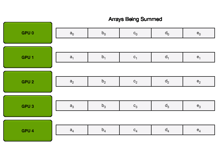
The next animation shows the AllGather step, where, at the end, each GPU obtains the full results of the AllReduce operation:
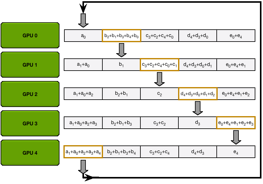
You may have noticed that each of the
There are two key things to keep in mind for AllReduce:
- The communication cost for AllReduce is approximately
2xK whenN (the number of GPUs) is large. - An AllReduce operation can be broken down into a reduce-scatter followed by an all-gather. The communication cost for these two operations is half that of the AllReduce, which is approximately
K .
As we can see this implementation can make efficient use of even a limited bandwidth between nodes.
We now have seen the main building block of distributed operations but before we see them in action let’s have a look at a special operation used for synchronization: the Barrier.
Barrier
The Barrier is a simple operation to synchronize all nodes. A barrier is not lifted until all nodes have reached it. Then only are they allowed to continue with further computations:

We can easily simulate delayed nodes by setting up a different sleep time on each node and see how long it takes for all of them to pass the barrier:
We can see that although the first rank didn’t sleep at all it also took it 2sec to pass the barrier:
We need to be careful with synchronizing all nodes like this, as this defeat the purpose of parallel independent operations and might thus slow down the whole processing. In many situations it can be just fine if a fast node already starts processing the next job as the fast node could be slower in a next iteration therefore evening out the delay over the whole process.
Before turning to practical distributed training implementations, let’s first solve a mystery: what the heck is NCCL?
NCCL: NVIDIA Collective Communications Library
When training large models on many GPUs we may sometimes strike gold but we will always encounter nickel (or NCCL 🥁)! What’s is that?
There are several libraries that implement collective communication and are support by PyTorch: there’s the classic MPI (Message Passing Interface), there’s Gloo by Meta, and finally there is `NCCL` (NVIDIA Collective Communications Library). They all provide similar functionality in terms of collective communication patterns but are optimized for different hardware setups; NCCL is designed to serve GPU-GPU communication efficiently while MPI and Gloo are setup for CPU-CPU or CPU-GPU communication. PyTorch provides a great guide to decide which one to use:
- GPU training: use NCCL
- CPU training: use Gloo
There are a few finer points in the decision tree that we leave to the reader to explore in the PyTorch guide referenced above.
Now that we covered the fundamental operations for distributed training and you should now be ready to follow the blog post easily.
A1: Distributed Training Profiling
Kernels
Let's begin by assuming for now that the kernels are already integrated into PyTorch. As a simple example, we can look at the Layer Normalization function implemented in PyTorch as torch.nn.functional.layer_norm. There are several methods to profile the kernel that underlies this function. The most straightforward approach might be to use the Python time module. However, since CUDA operations are asynchronous, measuring time with this method will only capture the overhead associated with launching the kernel in Python, rather than the actual execution time of the kernel itself.
To address this, we can utilize torch.cuda.Event for accurate timing and employ the torch.cuda.synchronize() directive to ensure we wait for the kernel execution to complete. This approach is demonstrated in the following snippet:
A more effective approach to profiling is to utilize the PyTorch Profiler, as explained previously. For example, consider the following code:
This would print aggregated profiling results sorted by the total CUDA time, and the output would be:

You can also try to inspect the trace as we previously mentioned on chrome://tracing/
💡 Tip
If you're new to this tool, you can navigate the trace by using the right and left arrow keys. Additionally, you can zoom in and out by holding the Alt key while scrolling left or right with your mouse.
After zooming in, you can observe the flow of operations when calling layer_norm in this trace:

The sequence begins in the CPU (the upper section) with aten::layer_norm, progressing to aten::native_layer_norm, and then transitioning to cudaLaunchKernel. From there, we move on to the GPU, where the vectorized_layer_norm_kernel kernel is called.
📝 Note
You can enable memory profiling by setting profile_memory to True in the profiler. However, this can lead to more complex traces.
While the PyTorch Profiler offers a quick performance overview, NVIDIA Nsight Compute (ncu) provides deeper insights into GPU performance, including detailed execution times and memory usage for each kernel. To run the profiler it's very simple:
Where layer_norm.py is a straightforward file that executes the layer normalization function. This command will generate log outputs, but a more effective way to visualize the results is by setting the output flag:
and open the file output.ncu-rep with Nsight Compute, you will have a view that looks like this:

With clear warnings about compute and memory utilization, and how to make the kernel better in balancing compute and memory and achieve maximal occupancy.
CPP extension
If the kernel you want to profile isn't already integrated into PyTorch, you can use PyTorch's cpp_extension module to easily compile and run custom CUDA code. The process is straightforward—just create your CUDA kernel in a .cu file, and use the load function from the cpp_extension module to load it in Python.
The .cu file would like this for a simple add kernel:
And the python file to load the kernel:
Using this method, you can profile the custom CUDA kernel just as we demonstrated earlier with PyTorch's profiler or NVIDIA tools.
A2: Typical Scales in LLM Training
Let's get a feel for the typical sizes of things in LLM training. When we talk about memory or compute, we're often counting "elements" - think of these as numbers in tensors. To get the actual memory in bytes, you'll need to multiply by the size of each number (e.g., 2 bytes for bf16, 4 bytes for fp32).
Here are some quick ballpark figures:
- Input tokens: For each batch, we process
seq \cdot mbs tokens, where mbs is the micro batch size and seq is the sequence length. - Activations (hidden states): For a single layer, the hidden state tensor is of size
seq \cdot mbs \cdot h elements. - Model weights and gradients: Each weight matrix in your model (like in linears) is about
h^2 elements. This is per weight matrix. Gradients have the same size as weights. - Optimizer states: For each weight matrix (of elements
h^2 ), if you're using an optimizer like Adam with mixed precision training, it keeps momentum and variance states in fp32 precision (2 \cdot h^2 ), plus master weights in fp32 (h^2 ). So total optimizer states will be around (6 \cdot h^2 ) per weight matrix. - Total model parameters: For each transformer block:
- Attention parameters:
- QKV projections:
3h^2 parameters - Output projection:
h^2 parameters
- QKV projections:
- MLP parameters with GLU:
- Gate and up projections:
8h^2 parameters (2 matrices of sizeh \times 4h ) - Down projection:
4h^2 parameters (1 matrix of size4h \times h )
- Gate and up projections:
- Total per block:
16h^2 with GLU MLPs, or12h^2 without GLU - For full model:
16h^2 \cdot num\_layers (with GLU) - Additional parameters:
- Input embeddings:
vocab\_size \cdot h - LM head:
vocab\_size \cdot h (if not tied with input embeddings) - Positional embeddings (if used):
max\_seq\_len \cdot h
- Input embeddings:
- Attention parameters:
- Forward and backward pass compute (FLOPs): A very rough estimate for the FLOPs in a forward pass is
2 \cdot num\_tokens \cdot num\_params . And backward pass compute is twice as that:4 \cdot num\_tokens \cdot num\_params .
A3: Math for Compute/Communication Overlap
Using the formulas from the previous section, we can estimate when computation and communication can effectively overlap in distributed training. Let's look at data parallelism (Zero-0) as an example.
Data Parallelism Communication Analysis
The total gradient size that needs to be communicated is:
- Gradients = Parameters ≈
num\_layers \cdot 16h^2
During backward pass, these gradients are communicated in buckets (default 25MB). The communication time to all-reduce each bucket is:
📝 Note
For bandwidth calculations, we use the bus bandwidth formulas from the NCCL documentation. These formulas account for the specific communication patterns when calculating effective bandwidth between GPUs.
The computation time for backward pass is:
For effective overlap, we need:
This ratio helps determine if communication will become a bottleneck in training. When the ratio is less than 1, communication can be fully overlapped with computation.
ZeRO-3 (FSDP) Communication Analysis
For ZeRO-3, parameters and gradients are sharded across GPUs. Let's analyze the communication pattern for a model with transformer blocks of size
- For each transformer block in forward pass:
- Allgather parameters:
16h^2/DP bytes per rank
- Allgather parameters:
- For each transformer block in backward pass:
- Allgather parameters:
16h^2/DP bytes per rank - Reducescatter gradients:
16h^2/DP bytes per rank
- Allgather parameters:
- Total communication per block:
3 \cdot 16h^2/DP bytes - Total communication for full model:
3 \cdot num\_layers \cdot 16h^2/DP bytes
The communication time for allgather operations is:
The computation time for forward pass of one decoder layer is:
For effective overlap between computation and communication, we need:
When this ratio is less than 1, the communication of parameters for the next layer can be hidden behind the computation of the current layer.
`TP Communication Analysis
For Tensor Parallel (TP), activations are sharded across GPUs during linears. Let's analyze the communication pattern:
- For each column linear in forward pass:
- Allgather activations:
seq \cdot mbs \cdot h/TP bytes per rank
- Allgather activations:
- For each column linear in backward pass:
- Reducescatter gradients:
seq \cdot mbs \cdot h/TP bytes per rank
- Reducescatter gradients:
- And vice-versa for row linears. Each transformer block has 2 column linears and 2 row linears.
- Total communication per block:
8 \cdot seq \cdot mbs \cdot h/TP bytes - Total communication for full model:
8 \cdot num\_layers \cdot seq \cdot mbs \cdot h/TP bytes
Let's analyze if we can overlap the allgather communication for one layer with the computation of the next linear. The communication time for allgather operations is:
While the computation time for the next linear (with parameters
For effective overlap, we want the communication time to be less than the compute time:
This ratio tells us whether we can successfully hide the allgather communication behind the computation of the next linear. Interestingly, the ratio only depends on the hidden size h and tensor parallelism degree TP, not on sequence length or batch size.
PP Communication Analysis
For Pipeline Parallel (PP), activations and gradients are communicated between pipeline stages. Let's analyze the communication pattern:
- For each microbatch in forward pass:
- Receive and send activations:
2 \cdot seq \cdot mbs \cdot h bytes
- Receive and send activations:
- For each microbatch in backward pass:
- Receive and send gradients:
2 \cdot seq \cdot mbs \cdot h bytes
- Receive and send gradients:
- Total communication per microbatch:
4 \cdot seq \cdot mbs \cdot h bytes - For gradient accumulation steps (gas), total communication:
4 \cdot gas \cdot seq \cdot mbs \cdot h bytes
Let's analyze if we can overlap the communication of activations/gradients with computation of the next transformer block. The computation time for transformer blocks in the next pipeline stage is:
While the communication time for P2P transfer is:
For effective overlap, we want:
Similar to TP, this ratio is independent of sequence length and batch size. It depends on the hidden size h, number of layers in the next pipeline stage, and the ratio of compute to P2P bandwidth capabilities of the hardware.